Simple Microscope Simulation - Spherical Inclusions¶

This notebook demonstrates simulating microscope imaging of a sample with multiple spherical inclusions using the simple_microscope function.

Overview¶

We create a 2D sample with ~50 randomly placed spherical inclusions:

Random positions across the field of view
Random radii between 50-500 pixels (25-250 µm)
Random refractive index contrast
Projected to 2D transmission function for imaging

Imports¶

In [1]:

import janssen as jns
import jax
import jax.numpy as jnp
import matplotlib.pyplot as plt
import numpy as np
import cmocean.cm as cmo
from matplotlib_scalebar.scalebar import ScaleBar
from matplotlib.patches import Circle

In [2]:

jns.__version__

Out [2]:

'2025.10.6'

In [3]:

%load_ext autoreload
%autoreload 2

Define Simulation Parameters¶

Same grid as USAF sample: 4096x4096 pixels at 0.5 µm pixel size.

In [4]:

pixel_size = 0.5e-6  # 0.5 microns
num_pixels = 4096  # Same as USAF sample
wavelength = 633e-9  # 633 nm (HeNe laser)

# Sphere parameters
num_spheres = 200
min_radius_pixels = 50  # Minimum radius in pixels
max_radius_pixels = 500  # Maximum radius in pixels

# Refractive indices - almost transparent (small contrast, no absorption)
n_background = 1.0 + 0.0j  # Air/vacuum background

# Random seed for reproducibility
np.random.seed(42)

print(f"Pixel size: {pixel_size * 1e6:.1f} microns")
print(f"Grid size: {num_pixels} x {num_pixels} pixels")
print(f"Field of view: {pixel_size * num_pixels * 1e3:.2f} mm")
print(f"Wavelength: {wavelength * 1e9:.0f} nm")
print(f"Number of spheres: {num_spheres}")
print(
    f"Radius range: {min_radius_pixels}-{max_radius_pixels} pixels ({min_radius_pixels * pixel_size * 1e6:.0f}-{max_radius_pixels * pixel_size * 1e6:.0f} µm)"
)

Pixel size: 0.5 microns
Grid size: 4096 x 4096 pixels
Field of view: 2.05 mm
Wavelength: 633 nm
Number of spheres: 200
Radius range: 50-500 pixels (25-250 µm)

1. Generate Random Sphere Parameters¶

Create random positions, radii, and refractive indices for all spheres.

In [5]:

# Generate uniformly distributed sphere positions using grid + jitter
# Create a grid covering the full image (spheres can be cut off at edges)
grid_size = int(
    np.ceil(np.sqrt(num_spheres))
)  # e.g., 8x8 grid for ~50 spheres

# No margin - spheres can extend to edges and be cut off
grid_spacing_y = num_pixels / grid_size
grid_spacing_x = num_pixels / grid_size

grid_y, grid_x = np.meshgrid(
    np.linspace(
        grid_spacing_y / 2, num_pixels - grid_spacing_y / 2, grid_size
    ),
    np.linspace(
        grid_spacing_x / 2, num_pixels - grid_spacing_x / 2, grid_size
    ),
)
grid_centers = np.stack([grid_y.ravel(), grid_x.ravel()], axis=1)

# Randomly select num_spheres positions from grid and add jitter
selected_indices = np.random.choice(
    len(grid_centers), num_spheres, replace=False
)
sphere_centers = grid_centers[selected_indices]

# Add jitter (up to 25% of grid spacing for more uniform look)
jitter_amount = 0.25 * min(grid_spacing_y, grid_spacing_x)
sphere_centers_y = sphere_centers[:, 0] + np.random.uniform(
    -jitter_amount, jitter_amount, num_spheres
)
sphere_centers_x = sphere_centers[:, 1] + np.random.uniform(
    -jitter_amount, jitter_amount, num_spheres
)

# Radii: uniform distribution between min and max
sphere_radii_pixels = np.random.uniform(
    min_radius_pixels, max_radius_pixels, num_spheres
)

# Refractive index - unique for each sphere, clustered values
# Bigger spheres are more transparent (smaller contrast), smaller spheres less transparent
# Normalize radius to [0, 1] range
radius_normalized = (sphere_radii_pixels - min_radius_pixels) / (
    max_radius_pixels - min_radius_pixels
)

# Base refractive index with small random variation for each sphere
# Real part: smaller spheres have higher contrast (n ~ 1.008), bigger spheres lower (n ~ 1.003)
# Add small unique variation to each
base_n_real = 1.003 + 0.005 * (
    1 - radius_normalized
)  # Inversely proportional to size
sphere_n_real = base_n_real + np.random.uniform(
    -0.0005, 0.0005, num_spheres
)  # Small unique variation

# Imaginary part: smaller spheres have more absorption, bigger spheres less
# Smaller spheres: κ ~ 0.0003, bigger spheres: κ ~ 0.00005
base_n_imag = 0.00005 + 0.00025 * (
    1 - radius_normalized
)  # Inversely proportional to size
sphere_n_imag = base_n_imag + np.random.uniform(
    -0.00002, 0.00002, num_spheres
)  # Small unique variation
sphere_n_imag = np.maximum(sphere_n_imag, 0)  # Ensure non-negative

sphere_n = sphere_n_real + 1j * sphere_n_imag

print(f"Generated {num_spheres} spheres with uniform distribution")
print(
    f"Grid: {grid_size}x{grid_size} = {grid_size**2} positions, selected {num_spheres}"
)
print(f"Grid spacing: {grid_spacing_y:.0f} x {grid_spacing_x:.0f} pixels")
print(
    f"Center Y range: {sphere_centers_y.min():.0f} to {sphere_centers_y.max():.0f} pixels"
)
print(
    f"Center X range: {sphere_centers_x.min():.0f} to {sphere_centers_x.max():.0f} pixels"
)
print(
    f"Radius range: {sphere_radii_pixels.min():.0f} to {sphere_radii_pixels.max():.0f} pixels"
)
print(
    f"Refractive index (real) range: {sphere_n_real.min():.5f} to {sphere_n_real.max():.5f}"
)
print(
    f"Absorption (imag) range: {sphere_n_imag.min():.6f} to {sphere_n_imag.max():.6f}"
)
print(
    f"Contrast (n-1) range: {(sphere_n_real-1).min():.5f} to {(sphere_n_real-1).max():.5f}"
)

Generated 200 spheres with uniform distribution
Grid: 15x15 = 225 positions, selected 200
Grid spacing: 273 x 273 pixels
Center Y range: 74 to 4025 pixels
Center X range: 96 to 4025 pixels
Radius range: 51 to 499 pixels
Refractive index (real) range: 1.00266 to 1.00821
Absorption (imag) range: 0.000035 to 0.000315
Contrast (n-1) range: 0.00266 to 0.00821

2. Create 2D Sample with Spherical Projections¶

For each sphere, we compute the 2D projection (optical path length through a sphere). For a sphere of radius R centered at origin, the path length at position (x,y) is: \(L(x,y) = 2\sqrt{R^2 - x^2 - y^2}\) for \(x^2 + y^2 < R^2\)

In [6]:

# Create 2D sample with projected spheres using vmap
# Create coordinate grids
y_coords = jnp.arange(num_pixels)
x_coords = jnp.arange(num_pixels)
yy, xx = jnp.meshgrid(y_coords, x_coords, indexing="ij")

# Wave number
k = 2 * jnp.pi / wavelength

# Convert sphere parameters to JAX arrays
centers_y = jnp.array(sphere_centers_y)
centers_x = jnp.array(sphere_centers_x)
radii = jnp.array(sphere_radii_pixels)
n_spheres_arr = jnp.array(sphere_n)


def compute_sphere_transmission(cy, cx, radius, n_sphere):
    """Compute transmission contribution from a single sphere."""
    # Distance from sphere center (in pixels)
    dist_sq = (yy - cy) ** 2 + (xx - cx) ** 2

    # Path length through sphere (in meters)
    # L = 2 * sqrt(R^2 - r^2) for r < R, else 0
    path_length_pixels = 2 * jnp.sqrt(jnp.maximum(radius**2 - dist_sq, 0))
    path_length_meters = path_length_pixels * pixel_size

    # Phase and amplitude from this sphere
    delta_n = n_sphere - n_background
    sphere_transmission = jnp.exp(1j * k * delta_n * path_length_meters)

    return sphere_transmission


# vmap over all spheres and multiply contributions together
all_transmissions = jax.vmap(compute_sphere_transmission)(
    centers_y, centers_x, radii, n_spheres_arr
)

# Product of all sphere transmissions (shape: num_pixels x num_pixels)
sample_transmission = jnp.prod(all_transmissions, axis=0)

print(f"Sample created using vmap!")
print(
    f"Amplitude range: {jnp.abs(sample_transmission).min():.4f} to {jnp.abs(sample_transmission).max():.4f}"
)
print(
    f"Phase range: {jnp.angle(sample_transmission).min():.4f} to {jnp.angle(sample_transmission).max():.4f} rad"
)

WARNING:2025-12-16 20:46:10,697:jax._src.xla_bridge:864: An NVIDIA GPU may be present on this machine, but a CUDA-enabled jaxlib is not installed. Falling back to cpu.

Sample created using vmap!
Amplitude range: 0.1303 to 1.0000
Phase range: -3.1416 to 3.1416 rad

In [7]:

# Create sample function
sphere_sample = jns.utils.make_sample_function(
    sample=sample_transmission,
    dx=pixel_size,
)

print(f"Sample shape: {sphere_sample.sample.shape}")
print(f"Sample dx: {sphere_sample.dx * 1e6:.2f} microns")

Sample shape: (4096, 4096)
Sample dx: 0.50 microns

In [8]:

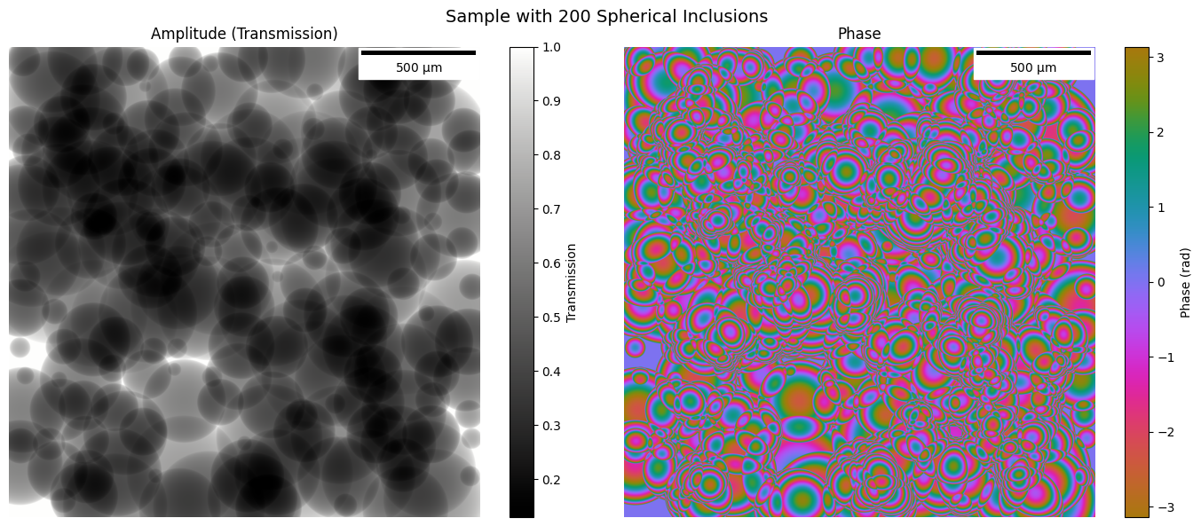
# Visualize the sample
fig, axes = plt.subplots(1, 2, figsize=(14, 6))

amp = jnp.abs(sphere_sample.sample)
phase = jnp.angle(sphere_sample.sample)

# Amplitude
im0 = axes[0].imshow(amp, cmap=cmo.gray)
axes[0].set_title("Amplitude (Transmission)")
scalebar = ScaleBar(sphere_sample.dx, "m", length_fraction=0.25, color="black")
axes[0].add_artist(scalebar)
axes[0].axis("off")
plt.colorbar(im0, ax=axes[0], label="Transmission")

# Phase
im1 = axes[1].imshow(phase, cmap=cmo.phase, vmin=-jnp.pi, vmax=jnp.pi)
axes[1].set_title("Phase")
scalebar = ScaleBar(sphere_sample.dx, "m", length_fraction=0.25, color="black")
axes[1].add_artist(scalebar)
axes[1].axis("off")
plt.colorbar(im1, ax=axes[1], label="Phase (rad)")

plt.suptitle(f"Sample with {num_spheres} Spherical Inclusions", fontsize=14)
plt.tight_layout()
plt.show()

../../_images/tutorials_Simulated_Microscopes_Spheres_12_0.png

3. Create Illumination Wavefront¶

In [9]:

illumination_size = 256  # Same as USAF notebook

lightwave = jns.models.plane_wave(
    wavelength=wavelength,
    dx=pixel_size,
    grid_size=(illumination_size, illumination_size),
    amplitude=1.0,
)

print(f"Illumination field shape: {lightwave.field.shape}")
print(f"Illumination wavelength: {lightwave.wavelength * 1e9:.0f} nm")
print(f"Illumination dx: {lightwave.dx * 1e6:.2f} microns")
print(f"Illumination FOV: {illumination_size * pixel_size * 1e6:.0f} microns")

Illumination field shape: (256, 256)
Illumination wavelength: 633 nm
Illumination dx: 0.50 microns
Illumination FOV: 128 microns

4. Set Microscope Parameters¶

In [10]:

# Microscope parameters
zoom_factor = 10.0  # 10x magnification
aperture_diameter = 1e-3  # 1 mm aperture
travel_distance = 0.1  # 150 mm to camera
detector_pixel_size = jnp.array(16e-6)  # 16 micron camera pixels

print(f"Zoom factor: {zoom_factor}x")
print(f"Aperture diameter: {aperture_diameter * 1e3:.1f} mm")
print(f"Travel distance: {travel_distance * 1e3:.0f} mm")
print(f"Detector pixel size: {detector_pixel_size * 1e6:.1f} µm")

Zoom factor: 10.0x
Aperture diameter: 1.0 mm
Travel distance: 100 mm
Detector pixel size: 16.0 µm

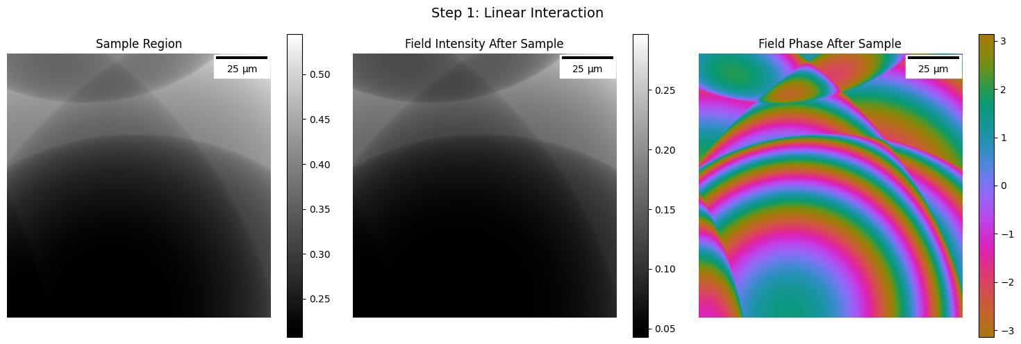
5. Step-by-Step Diffractogram Formation¶

Let’s visualize each step in the formation of a diffractogram:

Linear Interaction - Light interacts with the sample
Optical Zoom - Magnification by the objective lens
Circular Aperture - Limits the numerical aperture
Fraunhofer Propagation - Far-field propagation to the camera

In [11]:

# Cut sample at center for step-by-step visualization
center_pixel = num_pixels // 2
half_size = illumination_size // 2
sample_cut = sphere_sample.sample[
    center_pixel - half_size : center_pixel + half_size,
    center_pixel - half_size : center_pixel + half_size,
]

sample_region = jns.utils.make_sample_function(
    sample=sample_cut,
    dx=pixel_size,
)

print(f"Sample region shape: {sample_region.sample.shape}")

Sample region shape: (256, 256)

In [12]:

# Step 1: Linear Interaction - Light through sample
after_sample = jns.scopes.linear_interaction(
    sample=sample_region,
    light=lightwave,
)

print(f"After sample field shape: {after_sample.field.shape}")
print(f"After sample dx: {after_sample.dx * 1e6:.2f} microns")

# Visualize
fig, axes = plt.subplots(1, 3, figsize=(15, 5))

im0 = axes[0].imshow(jnp.abs(sample_region.sample), cmap=cmo.gray)
axes[0].set_title("Sample Region")
scalebar = ScaleBar(sample_region.dx, "m", length_fraction=0.25, color="black")
axes[0].add_artist(scalebar)
axes[0].axis("off")
plt.colorbar(im0, ax=axes[0])

im1 = axes[1].imshow(jnp.abs(after_sample.field) ** 2, cmap=cmo.gray)
axes[1].set_title("Field Intensity After Sample")
scalebar = ScaleBar(after_sample.dx, "m", length_fraction=0.25, color="black")
axes[1].add_artist(scalebar)
axes[1].axis("off")
plt.colorbar(im1, ax=axes[1])

im2 = axes[2].imshow(
    jnp.angle(after_sample.field), cmap=cmo.phase, vmin=-jnp.pi, vmax=jnp.pi
)
axes[2].set_title("Field Phase After Sample")
scalebar = ScaleBar(after_sample.dx, "m", length_fraction=0.25, color="black")
axes[2].add_artist(scalebar)
axes[2].axis("off")
plt.colorbar(im2, ax=axes[2])

plt.suptitle("Step 1: Linear Interaction", fontsize=14)
plt.tight_layout()
plt.show()

After sample field shape: (256, 256)
After sample dx: 0.50 microns

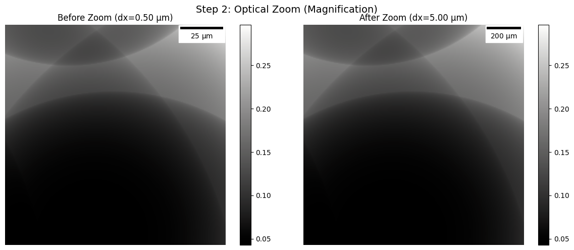
../../_images/tutorials_Simulated_Microscopes_Spheres_19_1.png

In [13]:

# Step 2: Optical Zoom - Magnification
zoomed_wave = jns.prop.optical_zoom(after_sample, zoom_factor)

print(f"Before zoom dx: {after_sample.dx * 1e6:.2f} microns")
print(f"After zoom dx: {zoomed_wave.dx * 1e6:.2f} microns")
print(f"Magnification achieved: {zoomed_wave.dx / after_sample.dx:.1f}x")

# Visualize
fig, axes = plt.subplots(1, 2, figsize=(12, 5))

im0 = axes[0].imshow(jnp.abs(after_sample.field) ** 2, cmap=cmo.gray)
axes[0].set_title(f"Before Zoom (dx={after_sample.dx*1e6:.2f} µm)")
scalebar = ScaleBar(after_sample.dx, "m", length_fraction=0.25, color="black")
axes[0].add_artist(scalebar)
axes[0].axis("off")
plt.colorbar(im0, ax=axes[0])

im1 = axes[1].imshow(jnp.abs(zoomed_wave.field) ** 2, cmap=cmo.gray)
axes[1].set_title(f"After Zoom (dx={zoomed_wave.dx*1e6:.2f} µm)")
scalebar = ScaleBar(zoomed_wave.dx, "m", length_fraction=0.25, color="black")
axes[1].add_artist(scalebar)
axes[1].axis("off")
plt.colorbar(im1, ax=axes[1])

plt.suptitle("Step 2: Optical Zoom (Magnification)", fontsize=14)
plt.tight_layout()
plt.show()

Before zoom dx: 0.50 microns
After zoom dx: 5.00 microns
Magnification achieved: 10.0x

../../_images/tutorials_Simulated_Microscopes_Spheres_20_1.png

In [14]:

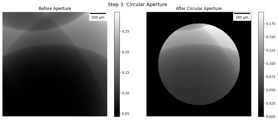
# Step 3: Circular Aperture - NA Limit
after_aperture = jns.optics.circular_aperture(
    zoomed_wave,
    diameter=aperture_diameter,
)

print(f"Aperture diameter: {aperture_diameter * 1e3:.1f} mm")

# Visualize
fig, axes = plt.subplots(1, 2, figsize=(12, 5))

im0 = axes[0].imshow(jnp.abs(zoomed_wave.field) ** 2, cmap=cmo.gray)
axes[0].set_title("Before Aperture")
scalebar = ScaleBar(zoomed_wave.dx, "m", length_fraction=0.25, color="black")
axes[0].add_artist(scalebar)
axes[0].axis("off")
plt.colorbar(im0, ax=axes[0])

im1 = axes[1].imshow(jnp.abs(after_aperture.field) ** 2, cmap=cmo.gray)
axes[1].set_title("After Circular Aperture")
scalebar = ScaleBar(
    after_aperture.dx, "m", length_fraction=0.25, color="black"
)
axes[1].add_artist(scalebar)
axes[1].axis("off")
plt.colorbar(im1, ax=axes[1])

plt.suptitle("Step 3: Circular Aperture", fontsize=14)
plt.tight_layout()
plt.show()

Aperture diameter: 1.0 mm

../../_images/tutorials_Simulated_Microscopes_Spheres_21_1.png

In [15]:

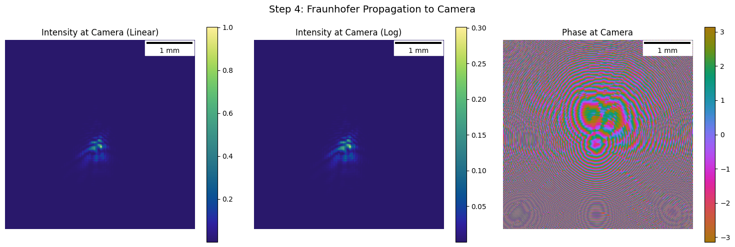
# Step 4: Fraunhofer Propagation - To Camera Plane
at_camera = jns.prop.fraunhofer_prop_scaled(
    after_aperture, travel_distance, output_dx=detector_pixel_size
)

print(f"Propagation distance: {travel_distance * 1e3:.0f} mm")
print(f"Camera plane dx: {at_camera.dx * 1e6:.2f} microns")

# Visualize
fig, axes = plt.subplots(1, 3, figsize=(15, 5))

im0 = axes[0].imshow(
    jns.optics.field_intensity(at_camera.field), cmap=cmo.haline
)
axes[0].set_title("Intensity at Camera (Linear)")
scalebar = ScaleBar(at_camera.dx, "m", length_fraction=0.25, color="black")
axes[0].add_artist(scalebar)
axes[0].axis("off")
plt.colorbar(im0, ax=axes[0])

im1 = axes[1].imshow(
    jnp.log10(1 + jns.optics.field_intensity(at_camera.field)), cmap=cmo.haline
)
axes[1].set_title("Intensity at Camera (Log)")
scalebar = ScaleBar(at_camera.dx, "m", length_fraction=0.25, color="black")
axes[1].add_artist(scalebar)
axes[1].axis("off")
plt.colorbar(im1, ax=axes[1])

im2 = axes[2].imshow(
    jnp.angle(at_camera.field), cmap=cmo.phase, vmin=-jnp.pi, vmax=jnp.pi
)
axes[2].set_title("Phase at Camera")
scalebar = ScaleBar(at_camera.dx, "m", length_fraction=0.25, color="black")
axes[2].add_artist(scalebar)
axes[2].axis("off")
plt.colorbar(im2, ax=axes[2])

plt.suptitle("Step 4: Fraunhofer Propagation to Camera", fontsize=14)
plt.tight_layout()
plt.show()

Propagation distance: 100 mm
Camera plane dx: 16.00 microns

../../_images/tutorials_Simulated_Microscopes_Spheres_22_1.png

In [16]:

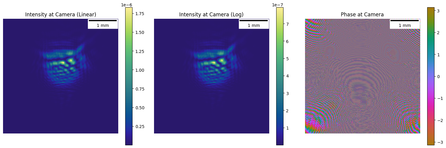
# Step 4: Fraunhofer Propagation - To Camera Plane
at_camera = jns.prop.fraunhofer_prop_scaled(
    after_aperture, travel_distance, output_dx=detector_pixel_size
)
at_camera_inv = jnp.fft.ifftshift(jnp.fft.ifft2(at_camera.field))

fig, axes = plt.subplots(1, 3, figsize=(15, 5))

im0 = axes[0].imshow(
    jns.optics.field_intensity(at_camera_inv), cmap=cmo.haline
)
axes[0].set_title("Intensity at Camera (Linear)")
scalebar = ScaleBar(at_camera.dx, "m", length_fraction=0.25, color="black")
axes[0].add_artist(scalebar)
axes[0].axis("off")
plt.colorbar(im0, ax=axes[0])

im1 = axes[1].imshow(
    jnp.log10(1 + jns.optics.field_intensity(at_camera_inv)), cmap=cmo.haline
)
axes[1].set_title("Intensity at Camera (Log)")
scalebar = ScaleBar(at_camera.dx, "m", length_fraction=0.25, color="black")
axes[1].add_artist(scalebar)
axes[1].axis("off")
plt.colorbar(im1, ax=axes[1])

im2 = axes[2].imshow(
    jnp.angle(at_camera_inv), cmap=cmo.phase, vmin=-jnp.pi, vmax=jnp.pi
)
axes[2].set_title("Phase at Camera")
scalebar = ScaleBar(at_camera.dx, "m", length_fraction=0.25, color="black")
axes[2].add_artist(scalebar)
axes[2].axis("off")
plt.colorbar(im2, ax=axes[2])

plt.tight_layout()
plt.show()

../../_images/tutorials_Simulated_Microscopes_Spheres_23_0.png

6. Compare with simple_diffractogram¶

Verify that the step-by-step approach matches the simple_diffractogram function.

In [17]:

# Generate single diffractogram using the combined function
diffractogram = jns.scopes.simple_diffractogram(
    sample_cut=sample_region,
    lightwave=lightwave,
    zoom_factor=zoom_factor,
    aperture_diameter=aperture_diameter,
    travel_distance=travel_distance,
    camera_pixel_size=detector_pixel_size,
)

print(f"Diffractogram shape: {diffractogram.image.shape}")
print(f"Diffractogram dx: {diffractogram.dx * 1e6:.2f} µm")

Diffractogram shape: (256, 256)
Diffractogram dx: 16.00 µm

In [18]:

# Compare manual pipeline with simple_diffractogram
fig, axes = plt.subplots(1, 2, figsize=(14, 6))

# Manual pipeline result
im0 = axes[0].imshow(
    jns.optics.field_intensity(at_camera.field), cmap=cmo.haline
)
axes[0].set_title("Manual Pipeline (Step by Step)")
scalebar = ScaleBar(at_camera.dx, "m", length_fraction=0.25, color="black")
axes[0].add_artist(scalebar)
axes[0].axis("off")
plt.colorbar(im0, ax=axes[0])

# Combined function result
im1 = axes[1].imshow(diffractogram.image, cmap=cmo.haline)
axes[1].set_title("simple_diffractogram Result")
scalebar = ScaleBar(diffractogram.dx, "m", length_fraction=0.25, color="black")
axes[1].add_artist(scalebar)
axes[1].axis("off")
plt.colorbar(im1, ax=axes[1])

plt.tight_layout()
plt.show()

# Verify they match
print(
    f"Max difference: {jnp.max(jnp.abs(jns.optics.field_intensity(at_camera.field) - diffractogram.image)):.2e}"
)

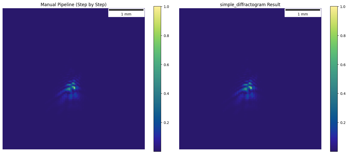
../../_images/tutorials_Simulated_Microscopes_Spheres_26_0.png

Max difference: 0.00e+00

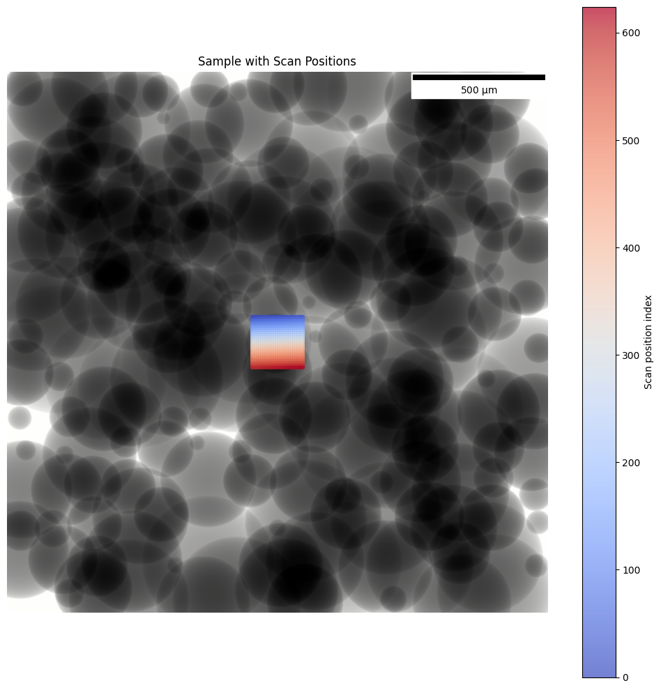
7. Full Microscope Simulation - Scanning¶

Create scan positions and run the full microscope simulation.

In [19]:

# Create scan positions centered on a region with spheres
scan_step = 8e-6  # 15 micron step size (same as USAF)
scan_pixel = scan_step / sphere_sample.dx

# Center of the sample
scope_center = jnp.array(
    [num_pixels // 2, num_pixels // 2]
)  # (x, y) in pixels

num_scan_x = 25
num_scan_y = 25

xx, yy = jnp.meshgrid(
    jnp.arange(num_scan_x) * scan_pixel - (num_scan_x - 1) * scan_pixel / 2,
    jnp.arange(num_scan_y) * scan_pixel - (num_scan_y - 1) * scan_pixel / 2,
)
x_positions = xx + scope_center[0]
y_positions = yy + scope_center[1]
positions = jnp.stack([x_positions.ravel(), y_positions.ravel()], axis=1)

print(f"Scan step: {scan_step * 1e6:.0f} µm ({scan_pixel:.1f} pixels)")
print(f"Number of scan positions: {len(positions)}")
print(f"Scan grid: {num_scan_x} x {num_scan_y}")
print(
    f"Total scan area: {(num_scan_x-1) * scan_step * 1e6:.0f} x {(num_scan_y-1) * scan_step * 1e6:.0f} µm"
)

Scan step: 8 µm (16.0 pixels)
Number of scan positions: 625
Scan grid: 25 x 25
Total scan area: 192 x 192 µm

In [20]:

# Visualize scan positions on sample
fig, ax = plt.subplots(1, 1, figsize=(10, 10))

im = ax.imshow(jnp.abs(sphere_sample.sample), cmap=cmo.gray)
ax.set_title("Sample with Scan Positions")
scalebar = ScaleBar(sphere_sample.dx, "m", length_fraction=0.25, color="black")
ax.add_artist(scalebar)

# Add scan positions as colored dots
scatter = ax.scatter(
    positions[:, 0],
    positions[:, 1],
    c=jnp.arange(len(positions)),
    cmap="coolwarm",
    s=10,
    alpha=0.7,
    marker="o",
)
plt.colorbar(scatter, ax=ax, label="Scan position index")
ax.axis("off")

plt.tight_layout()
plt.show()

../../_images/tutorials_Simulated_Microscopes_Spheres_29_0.png

In [21]:

# Run simple_microscope with all scan positions
positions_meters = positions * sphere_sample.dx

microscope_data = jns.scopes.simple_microscope(
    sample=sphere_sample,
    positions=positions_meters,
    lightwave=lightwave,
    zoom_factor=zoom_factor,
    aperture_diameter=aperture_diameter,
    travel_distance=travel_distance,
    camera_pixel_size=detector_pixel_size,
)

print(f"Microscope data shape: {microscope_data.image_data.shape}")
print(f"Number of diffractograms: {microscope_data.image_data.shape[0]}")
print(f"Diffractogram size: {microscope_data.image_data.shape[1:]}")
print(f"Camera pixel size: {microscope_data.dx * 1e6:.2f} µm")

Microscope data shape: (625, 256, 256)
Number of diffractograms: 625
Diffractogram size: (256, 256)
Camera pixel size: 16.00 µm

In [22]:

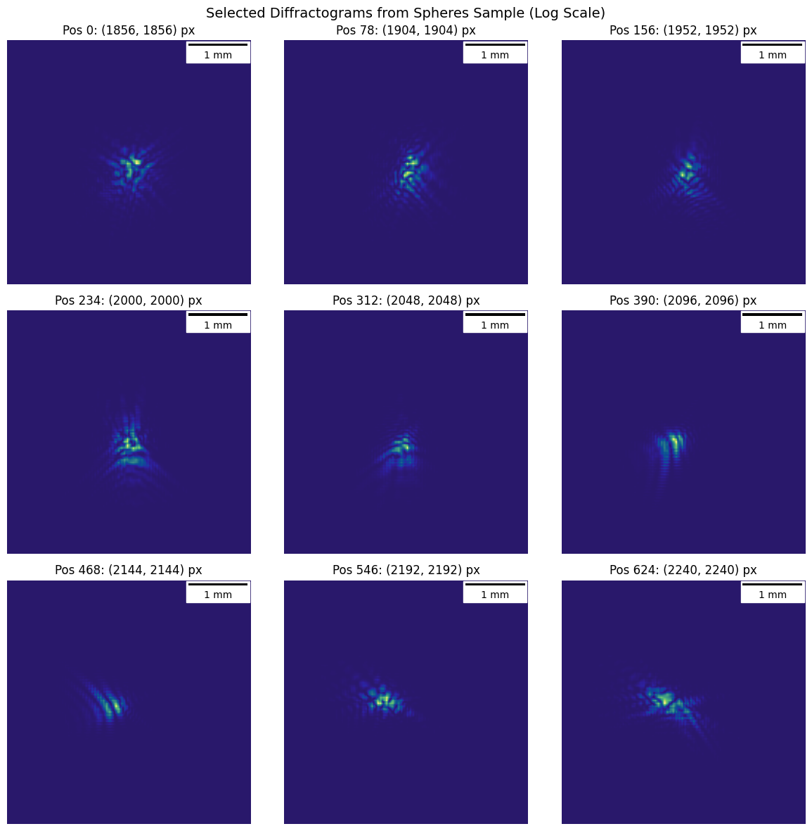
# Visualize a subset of diffractograms (9 evenly spaced)
fig, axes = plt.subplots(3, 3, figsize=(12, 12))

indices = jnp.linspace(0, len(positions) - 1, 9).astype(int)

for i, ax in enumerate(axes.flat):
    idx = int(indices[i])
    im = ax.imshow(
        jnp.log10(microscope_data.image_data[idx] + 1), cmap=cmo.haline
    )
    pos = positions[idx]
    ax.set_title(f"Pos {idx}: ({pos[0]:.0f}, {pos[1]:.0f}) px")
    scalebar = ScaleBar(
        microscope_data.dx, "m", length_fraction=0.25, color="black"
    )
    ax.add_artist(scalebar)
    ax.axis("off")

plt.suptitle(
    "Selected Diffractograms from Spheres Sample (Log Scale)", fontsize=14
)
plt.tight_layout()
plt.show()

../../_images/tutorials_Simulated_Microscopes_Spheres_31_0.png

In [23]:

fig, axes = plt.subplots(1, 3, figsize=(18, 6))
axes[0].imshow(jnp.log10(1 + microscope_data.image_data[64]), cmap=cmo.haline)
axes[1].imshow(jnp.log10(1 + microscope_data.image_data[65]), cmap=cmo.haline)
axes[2].imshow(jnp.log10(1 + microscope_data.image_data[66]), cmap=cmo.haline)
plt.show()

print("Diffractogram at pos 0 sum:", microscope_data.image_data[64].sum())
print("Diffractogram at pos 1 sum:", microscope_data.image_data[65].sum())
print(
    "Are they identical?",
    jnp.allclose(
        microscope_data.image_data[64], microscope_data.image_data[65]
    ),
)

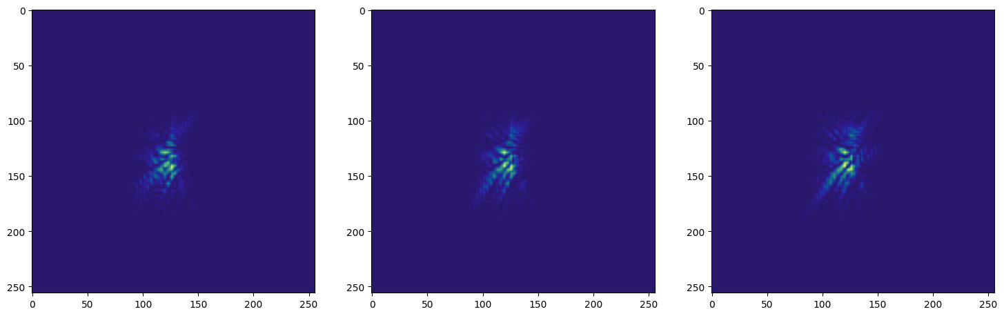
../../_images/tutorials_Simulated_Microscopes_Spheres_32_0.png

Diffractogram at pos 0 sum: 422.4509078399198
Diffractogram at pos 1 sum: 455.16915398686547
Are they identical? False

In [24]:

print("Experimental data shape:", microscope_data.image_data.shape)
print("Experimental positions shape:", microscope_data.positions.shape)
print("First few positions (meters):", microscope_data.positions[:5])
print(
    "Position range X:",
    microscope_data.positions[:, 0].min(),
    "to",
    microscope_data.positions[:, 0].max(),
)
print(
    "Position range Y:",
    microscope_data.positions[:, 1].min(),
    "to",
    microscope_data.positions[:, 1].max(),
)

Experimental data shape: (625, 256, 256)
Experimental positions shape: (625, 2)
First few positions (meters): [[0.000928 0.000928]
 [0.000936 0.000928]
 [0.000944 0.000928]
 [0.000952 0.000928]
 [0.00096  0.000928]]
Position range X: 0.000928 to 0.00112
Position range Y: 0.000928 to 0.00112

8. Ptychographic Reconstruction¶

Now we’ll use the ptychography algorithm to reconstruct both the sample and probe from the diffractogram data.

In [25]:

# Create ptychography parameters (optimization only)
ptycho_params = jns.utils.make_ptychography_params(
    camera_pixel_size=detector_pixel_size,
    num_iterations=40,
    learning_rate=1e-4,
    loss_type=0,  # 0=mse, 1=mae, 2=poisson
    optimizer_type=0,  # 0=adam, 1=adagrad, 2=rmsprop, 3=sgd
)

print(f"Camera pixel size: {ptycho_params.camera_pixel_size * 1e6:.1f} µm")
print(f"Learning rate: {ptycho_params.learning_rate}")
print(f"Num iterations: {ptycho_params.num_iterations}")
print(f"Loss type: {ptycho_params.loss_type} (0=mse)")
print(f"Optimizer type: {ptycho_params.optimizer_type} (0=adam)")

Camera pixel size: 16.0 µm
Learning rate: 0.0001
Num iterations: 40
Loss type: 0 (0=mse)
Optimizer type: 0 (0=adam)

In [26]:

# Initialize reconstruction by running microscope model in reverse
initial_reconstruction = jns.invert.init_simple_microscope(
    experimental_data=microscope_data,
    probe_lightwave=lightwave,
    zoom_factor=zoom_factor,
    aperture_diameter=aperture_diameter,
    travel_distance=travel_distance,
    camera_pixel_size=detector_pixel_size,
)

print(f"Initialized reconstruction!")
print(f"Initial sample shape: {initial_reconstruction.sample.sample.shape}")
print(
    f"Translated positions shape: {initial_reconstruction.translated_positions.shape}"
)
print(f"Initial MSE loss: {initial_reconstruction.losses[0, 1]:.6f}")

Initialized reconstruction!
Initial sample shape: (896, 896)
Translated positions shape: (625, 2)
Initial MSE loss: 0.234304

In [27]:

# Visualize initial reconstruction (sanity check before optimization)
fig, axes = plt.subplots(1, 2, figsize=(14, 6))

init_amp = jnp.abs(initial_reconstruction.sample.sample)
init_phase = jnp.angle(initial_reconstruction.sample.sample)

# Amplitude
im0 = axes[0].imshow(init_amp, cmap=cmo.gray)
axes[0].set_title("Initial Sample - Amplitude")
scalebar = ScaleBar(
    initial_reconstruction.sample.dx, "m", length_fraction=0.25, color="black"
)
axes[0].add_artist(scalebar)
axes[0].axis("off")
plt.colorbar(im0, ax=axes[0], label="Amplitude")

# Phase
im1 = axes[1].imshow(init_phase, cmap=cmo.phase, vmin=-jnp.pi, vmax=jnp.pi)
axes[1].set_title("Initial Sample - Phase")
scalebar = ScaleBar(
    initial_reconstruction.sample.dx, "m", length_fraction=0.25, color="black"
)
axes[1].add_artist(scalebar)
axes[1].axis("off")
plt.colorbar(im1, ax=axes[1], label="Phase (rad)")

plt.suptitle(
    f"Initial Reconstruction (MSE: {initial_reconstruction.losses[0, 1]:.4f})",
    fontsize=14,
)
plt.tight_layout()
plt.show()

../../_images/tutorials_Simulated_Microscopes_Spheres_37_0.png

In [28]:

center = jnp.astype(0.5 * jnp.asarray(init_amp.shape), jnp.int32)
pad = jnp.astype(
    jnp.amin(
        initial_reconstruction.translated_positions
        / initial_reconstruction.sample.dx
    ),
    jnp.int32,
)
print(
    f"The intensity at the center of the initial reconstruction is {init_amp[center[0]+2, center[1]+2]:.2e}"
)
print(f"The intensity at the top left corner is {init_amp[pad, pad]:.2e}")

The intensity at the center of the initial reconstruction is 6.49e-01
The intensity at the top left corner is 6.10e-01

In [29]:

# Run ptychographic reconstruction
reconstruction = jns.invert.simple_microscope_ptychography(
    experimental_data=microscope_data,
    reconstruction=initial_reconstruction,
    params=ptycho_params,
)

print(f"Reconstruction complete!")
print(f"Reconstructed sample shape: {reconstruction.sample.sample.shape}")
print(f"Reconstructed probe shape: {reconstruction.lightwave.field.shape}")
print(f"Final loss: {reconstruction.losses[-1, 1]:.6f}")

Reconstruction complete!
Reconstructed sample shape: (896, 896)
Reconstructed probe shape: (256, 256)
Final loss: 0.234056

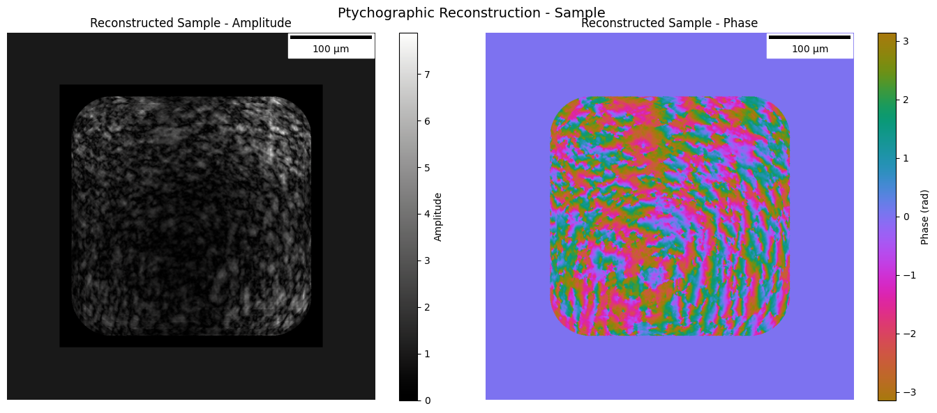
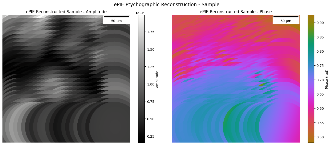
Visualize Reconstruction Results¶

In [30]:

reconstruction.sample.sample.shape

Out [30]:

(896, 896)

In [31]:

# Visualize reconstructed sample
fig, axes = plt.subplots(1, 2, figsize=(14, 6))

recon_amp = jnp.abs(reconstruction.sample.sample)
recon_phase = jnp.angle(reconstruction.sample.sample)

# Amplitude
im0 = axes[0].imshow(
    recon_amp, vmin=recon_amp.min(), vmax=recon_amp.max(), cmap=cmo.gray
)
axes[0].set_title("Reconstructed Sample - Amplitude")
scalebar = ScaleBar(
    reconstruction.sample.dx, "m", length_fraction=0.25, color="black"
)
axes[0].add_artist(scalebar)
axes[0].axis("off")
plt.colorbar(im0, ax=axes[0], label="Amplitude")

# Phase
im1 = axes[1].imshow(recon_phase, cmap=cmo.phase, vmin=-jnp.pi, vmax=jnp.pi)
axes[1].set_title("Reconstructed Sample - Phase")
scalebar = ScaleBar(
    reconstruction.sample.dx, "m", length_fraction=0.25, color="black"
)
axes[1].add_artist(scalebar)
axes[1].axis("off")
plt.colorbar(im1, ax=axes[1], label="Phase (rad)")

plt.suptitle("Ptychographic Reconstruction - Sample", fontsize=14)
plt.tight_layout()
plt.show()

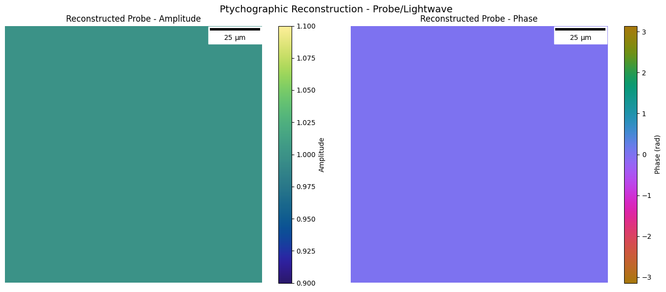
../../_images/tutorials_Simulated_Microscopes_Spheres_42_0.png

In [32]:

# Visualize reconstructed probe
fig, axes = plt.subplots(1, 2, figsize=(14, 6))

probe_amp = jnp.abs(reconstruction.lightwave.field)
probe_phase = jnp.angle(reconstruction.lightwave.field)

# Amplitude
im0 = axes[0].imshow(probe_amp, cmap=cmo.haline)
axes[0].set_title("Reconstructed Probe - Amplitude")
scalebar = ScaleBar(
    reconstruction.lightwave.dx, "m", length_fraction=0.25, color="black"
)
axes[0].add_artist(scalebar)
axes[0].axis("off")
plt.colorbar(im0, ax=axes[0], label="Amplitude")

# Phase
im1 = axes[1].imshow(probe_phase, cmap=cmo.phase, vmin=-jnp.pi, vmax=jnp.pi)
axes[1].set_title("Reconstructed Probe - Phase")
scalebar = ScaleBar(
    reconstruction.lightwave.dx, "m", length_fraction=0.25, color="black"
)
axes[1].add_artist(scalebar)
axes[1].axis("off")
plt.colorbar(im1, ax=axes[1], label="Phase (rad)")

plt.suptitle("Ptychographic Reconstruction - Probe/Lightwave", fontsize=14)
plt.tight_layout()
plt.show()

../../_images/tutorials_Simulated_Microscopes_Spheres_43_0.png

In [33]:

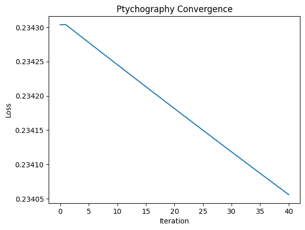
# Visualize evolution of loss
plt.plot(reconstruction.losses[:, 0], reconstruction.losses[:, 1])
plt.xlabel("Iteration")
plt.ylabel("Loss")
plt.title("Ptychography Convergence")

Out [33]:

Text(0.5, 1.0, 'Ptychography Convergence')

../../_images/tutorials_Simulated_Microscopes_Spheres_44_1.png

In [34]:

# Print final optimized parameters
print("Final Optimized Parameters:")
print(f"  Zoom factor: {reconstruction.zoom_factor:.4f} (true: {zoom_factor})")
print(
    f"  Aperture diameter: {reconstruction.aperture_diameter * 1e3:.4f} mm (true: {aperture_diameter * 1e3:.1f} mm)"
)
print(
    f"  Travel distance: {reconstruction.travel_distance * 1e3:.4f} mm (true: {travel_distance * 1e3:.0f} mm)"
)
if reconstruction.aperture_center is not None:
    print(f"  Aperture center: {reconstruction.aperture_center}")

Final Optimized Parameters:
  Zoom factor: 10.0000 (true: 10.0)
  Aperture diameter: 1.0000 mm (true: 1.0 mm)
  Travel distance: 100.0000 mm (true: 100 mm)
  Aperture center: [0. 0.]

In [35]:

print(
    "Sample amplitude range:",
    jnp.abs(reconstruction.sample.sample).min(),
    jnp.abs(reconstruction.sample.sample).max(),
)
print(
    "Sample phase range:",
    jnp.angle(reconstruction.sample.sample).min(),
    jnp.angle(reconstruction.sample.sample).max(),
)
print(
    "Probe amplitude range:",
    jnp.abs(reconstruction.lightwave.field).min(),
    jnp.abs(reconstruction.lightwave.field).max(),
)
print(
    "Probe phase range:",
    jnp.angle(reconstruction.lightwave.field).min(),
    jnp.angle(reconstruction.lightwave.field).max(),
)

Sample amplitude range: 0.0 7.887381589954676
Sample phase range: -3.141566730876553 3.1415664897289357
Probe amplitude range: 1.0 1.0
Probe phase range: 0.0 0.0

8. ePIE Reconstruction¶

Now let’s run the extended PIE (ePIE) algorithm on the data. We run ePIE first as it’s often faster to converge for ptychography problems.

In [36]:

# ePIE parameters - using dedicated EpieParams type
# effective_dx: desired reconstruction pixel size (user choice)
# This determines the resolution of the reconstructed sample
epie_params = jns.utils.make_epie_params(
    effective_dx=0.5e-6,  # 1.6 µm pixels (user choice for resolution)
    num_iterations=60,  # ePIE iterations (sweeps over all positions)
    alpha=1.0,  # Object update step size (0.5-1.0)
    beta=0.0,  # Probe update step size (0 = freeze probe)
    padding=32,  # Extra padding around scan region
)

print(f"ePIE Parameters:")
print(f"  Effective dx: {float(epie_params.effective_dx) * 1e6:.2f} µm")
print(f"  Num iterations: {int(epie_params.num_iterations)}")
print(f"  Alpha (object step): {float(epie_params.alpha)}")
print(f"  Beta (probe step): {float(epie_params.beta)}")
print(f"  Padding: {int(epie_params.padding)} pixels")

ePIE Parameters:
  Effective dx: 0.50 µm
  Num iterations: 60
  Alpha (object step): 1.0
  Beta (probe step): 0.0
  Padding: 32 pixels

In [37]:

# Initialize ePIE data directly using init_simple_epie
# This preprocesses the data: rescales camera images, creates probe with aperture,
# and converts positions to pixels centered at (0,0)
epie_data = jns.invert.init_simple_epie(
    experimental_data=microscope_data,
    effective_dx=float(epie_params.effective_dx),
    wavelength=wavelength,
    zoom_factor=zoom_factor,
    aperture_diameter=aperture_diameter,
    travel_distance=travel_distance,
    camera_pixel_size=detector_pixel_size,
    padding=int(epie_params.padding),
)

print(f"ePIE Data initialized:")
print(f"  Sample shape: {epie_data.sample.shape}")
print(f"  Probe shape: {epie_data.probe.shape}")
print(f"  Diffraction patterns shape: {epie_data.diffraction_patterns.shape}")
print(f"  Positions shape: {epie_data.positions.shape}")
print(f"  Effective dx: {float(epie_data.effective_dx) * 1e6:.2f} µm")
print(
    f"  Positions centered at: ({float(jnp.mean(epie_data.positions[:, 0])):.1f}, {float(jnp.mean(epie_data.positions[:, 1])):.1f}) px"
)

ePIE Data initialized:
  Sample shape: (649, 649)
  Probe shape: (649, 649)
  Diffraction patterns shape: (625, 649, 649)
  Positions shape: (625, 2)
  Effective dx: 0.50 µm
  Positions centered at: (0.0, 0.0) px

In [38]:

# Run ePIE core algorithm (pure pixel-space computation)
from janssen.invert.ptychography import _sm_epie_core

iterations = jnp.arange(int(epie_params.num_iterations), dtype=jnp.int64)
epie_result = _sm_epie_core(
    epie_data=epie_data,
    iterations=iterations,
    alpha=float(epie_params.alpha),
    beta=float(epie_params.beta),
)
epie_result.sample.block_until_ready()

print(f"ePIE Reconstruction complete!")
print(f"Final sample shape: {epie_result.sample.shape}")
print(f"Final probe shape: {epie_result.probe.shape}")

ePIE Reconstruction complete!
Final sample shape: (649, 649)
Final probe shape: (649, 649)

In [39]:

# Visualize ePIE reconstructed sample
fig, axes = plt.subplots(1, 2, figsize=(14, 6))
pad = 70
epie_amp = jnp.abs(epie_result.sample[pad:-pad, pad:-pad])
epie_phase = jnp.angle(epie_result.sample[pad:-pad, pad:-pad])

# Amplitude
im0 = axes[0].imshow(
    epie_amp, vmin=epie_amp.min(), vmax=epie_amp.max(), cmap=cmo.gray
)
axes[0].set_title("ePIE Reconstructed Sample - Amplitude")
scalebar = ScaleBar(
    float(epie_params.effective_dx), "m", length_fraction=0.25, color="black"
)
axes[0].add_artist(scalebar)
axes[0].axis("off")
plt.colorbar(im0, ax=axes[0], label="Amplitude")

# Phase
im1 = axes[1].imshow(
    epie_phase, cmap=cmo.phase, vmin=epie_phase.min(), vmax=epie_phase.max()
)
axes[1].set_title("ePIE Reconstructed Sample - Phase")
scalebar = ScaleBar(
    float(epie_params.effective_dx), "m", length_fraction=0.25, color="black"
)
axes[1].add_artist(scalebar)
axes[1].axis("off")
plt.colorbar(im1, ax=axes[1], label="Phase (rad)")

plt.suptitle("ePIE Ptychographic Reconstruction - Sample", fontsize=14)
plt.tight_layout()
plt.show()

../../_images/tutorials_Simulated_Microscopes_Spheres_51_0.png

Compare Gradient-Based vs ePIE Reconstruction¶

In [40]:

# Convergence plot for gradient-based method only
# Note: ePIE doesn't track per-iteration losses in this implementation
fig, ax = plt.subplots(1, 1, figsize=(10, 6))

# Gradient-based (Adam)
ax.plot(
    reconstruction.losses[:, 0],
    reconstruction.losses[:, 1],
    "b-",
    linewidth=2,
    label=f"Adam ({int(ptycho_params.num_iterations)} iters)",
)

ax.set_xlabel("Iteration", fontsize=12)
ax.set_ylabel("MSE Loss", fontsize=12)
ax.set_title("Reconstruction Convergence: Gradient-Based (Adam)", fontsize=14)
ax.legend(fontsize=11)
ax.grid(True, alpha=0.3)
ax.set_yscale("log")

plt.tight_layout()
plt.show()

print(
    f"\nFinal Gradient-Based (Adam) Loss: {reconstruction.losses[-1, 1]:.6f}"
)

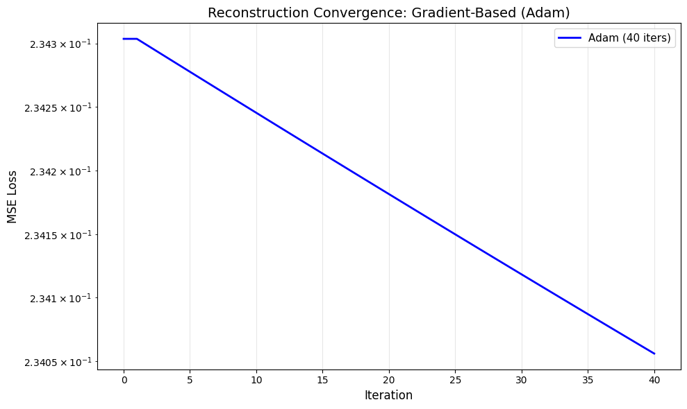
../../_images/tutorials_Simulated_Microscopes_Spheres_53_0.png


Final Gradient-Based (Adam) Loss: 0.234056

In [41]:

# Side-by-side comparison of reconstructed samples
fig, axes = plt.subplots(2, 2, figsize=(14, 12))

crop = slice(192, -192)

# Gradient-based amplitude
im00 = axes[0, 0].imshow(
    jnp.abs(reconstruction.sample.sample)[crop, crop], cmap=cmo.gray
)
axes[0, 0].set_title("Gradient (Adam) - Amplitude")
scalebar = ScaleBar(
    reconstruction.sample.dx, "m", length_fraction=0.25, color="black"
)
axes[0, 0].add_artist(scalebar)
axes[0, 0].axis("off")
plt.colorbar(im00, ax=axes[0, 0])

# ePIE amplitude - note: epie_result.sample is the raw array, use epie_params.effective_dx for scale
im01 = axes[0, 1].imshow(jnp.abs(epie_result.sample), cmap=cmo.gray)
axes[0, 1].set_title("ePIE - Amplitude")
scalebar = ScaleBar(
    float(epie_params.effective_dx), "m", length_fraction=0.25, color="black"
)
axes[0, 1].add_artist(scalebar)
axes[0, 1].axis("off")
plt.colorbar(im01, ax=axes[0, 1])

# Gradient-based phase
im10 = axes[1, 0].imshow(
    jnp.angle(reconstruction.sample.sample)[crop, crop],
    cmap=cmo.phase,
    vmin=-jnp.pi,
    vmax=jnp.pi,
)
axes[1, 0].set_title("Gradient (Adam) - Phase")
scalebar = ScaleBar(
    reconstruction.sample.dx, "m", length_fraction=0.25, color="black"
)
axes[1, 0].add_artist(scalebar)
axes[1, 0].axis("off")
plt.colorbar(im10, ax=axes[1, 0])

# ePIE phase
im11 = axes[1, 1].imshow(
    jnp.angle(epie_result.sample), cmap=cmo.phase, vmin=-jnp.pi, vmax=jnp.pi
)
axes[1, 1].set_title("ePIE - Phase")
scalebar = ScaleBar(
    float(epie_params.effective_dx), "m", length_fraction=0.25, color="black"
)
axes[1, 1].add_artist(scalebar)
axes[1, 1].axis("off")
plt.colorbar(im11, ax=axes[1, 1])

plt.suptitle(
    "Sample Reconstruction Comparison: Gradient-Based vs ePIE", fontsize=14
)
plt.tight_layout()
plt.show()

print(f"\nePIE sample shape: {epie_result.sample.shape}")
print(f"Adam sample shape: {reconstruction.sample.sample.shape}")

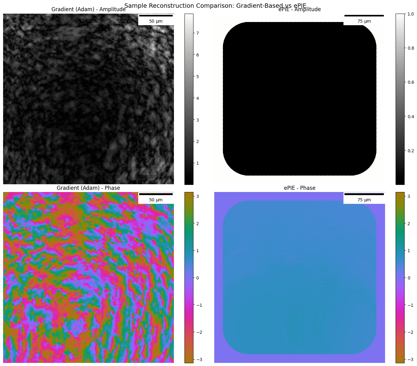
../../_images/tutorials_Simulated_Microscopes_Spheres_54_0.png


ePIE sample shape: (649, 649)
Adam sample shape: (896, 896)

In [42]:

# Compare reconstructed probes
fig, axes = plt.subplots(2, 2, figsize=(14, 12))

# Gradient-based probe amplitude
im00 = axes[0, 0].imshow(
    jnp.abs(reconstruction.lightwave.field), cmap=cmo.haline
)
axes[0, 0].set_title("Gradient (Adam) - Probe Amplitude")
scalebar = ScaleBar(
    reconstruction.lightwave.dx, "m", length_fraction=0.25, color="black"
)
axes[0, 0].add_artist(scalebar)
axes[0, 0].axis("off")
plt.colorbar(im00, ax=axes[0, 0])

# ePIE probe amplitude - note: epie_result.probe is the raw array
im01 = axes[0, 1].imshow(jnp.abs(epie_result.probe), cmap=cmo.haline)
axes[0, 1].set_title("ePIE - Probe Amplitude")
scalebar = ScaleBar(
    float(epie_params.effective_dx), "m", length_fraction=0.25, color="black"
)
axes[0, 1].add_artist(scalebar)
axes[0, 1].axis("off")
plt.colorbar(im01, ax=axes[0, 1])

# Gradient-based probe phase
im10 = axes[1, 0].imshow(
    jnp.angle(reconstruction.lightwave.field),
    cmap=cmo.phase,
    vmin=-jnp.pi,
    vmax=jnp.pi,
)
axes[1, 0].set_title("Gradient (Adam) - Probe Phase")
scalebar = ScaleBar(
    reconstruction.lightwave.dx, "m", length_fraction=0.25, color="black"
)
axes[1, 0].add_artist(scalebar)
axes[1, 0].axis("off")
plt.colorbar(im10, ax=axes[1, 0])

# ePIE probe phase
im11 = axes[1, 1].imshow(
    jnp.angle(epie_result.probe), cmap=cmo.phase, vmin=-jnp.pi, vmax=jnp.pi
)
axes[1, 1].set_title("ePIE - Probe Phase")
scalebar = ScaleBar(
    float(epie_params.effective_dx), "m", length_fraction=0.25, color="black"
)
axes[1, 1].add_artist(scalebar)
axes[1, 1].axis("off")
plt.colorbar(im11, ax=axes[1, 1])

plt.suptitle(
    "Probe Reconstruction Comparison: Gradient-Based vs ePIE", fontsize=14
)
plt.tight_layout()
plt.show()

print(f"\nePIE probe shape: {epie_result.probe.shape}")
print(f"Adam probe shape: {reconstruction.lightwave.field.shape}")
print(
    f"\nNote: ePIE probe update controlled by beta={float(epie_params.beta)} (0=frozen)."
)

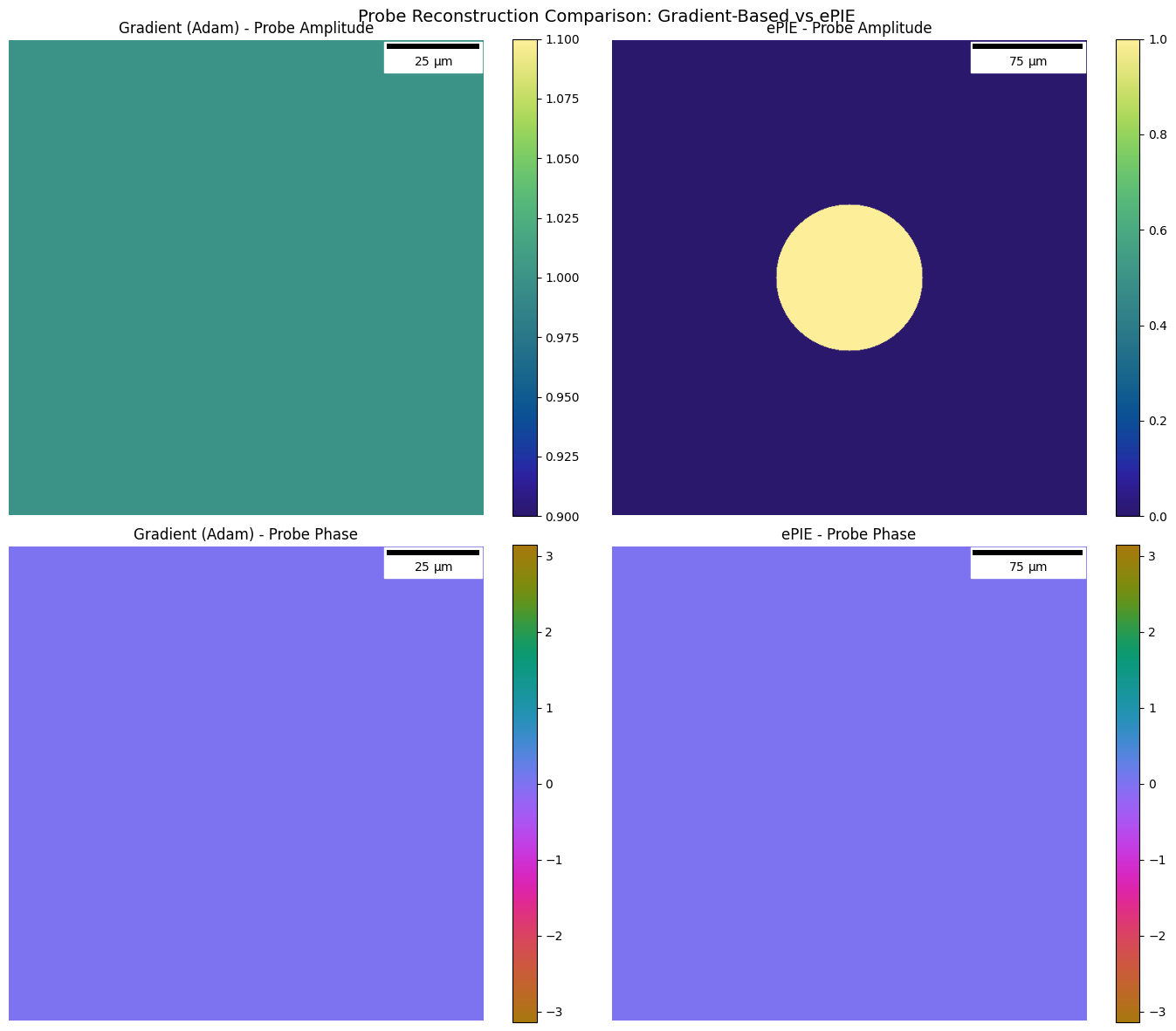
../../_images/tutorials_Simulated_Microscopes_Spheres_55_0.png


ePIE probe shape: (649, 649)
Adam probe shape: (256, 256)

Note: ePIE probe update controlled by beta=0.0 (0=frozen).