Create a diffractogram
Imports
Import the necessary packages. We import janssen as jns.
In [1]:
import janssen as jns
import jax
import jax.numpy as jnp
import matplotlib.pyplot as plt
import numpy as np
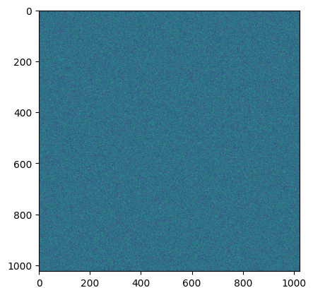
Generate a random image from Numpy, to be used as the lightwave.
In [2]:
random_image = (
    np.abs(np.reshape(np.random.randn(1024**2), (1024, 1024)))
) ** 0.5
plt.imshow(random_image)
Out [2]:
<matplotlib.image.AxesImage at 0x7f9146e5bdd0>
JIT compile the function(s) to be used.
In [3]:
make_optical_wavefront = jax.jit(jns.utils.make_optical_wavefront)
make_sample_function = jax.jit(jns.utils.make_sample_function)
linear_interaction = jax.jit(jns.scopes.linear_interaction)
optical_zoom = jax.jit(jns.prop.optical_zoom)
circular_aperture = jax.jit(jns.optics.circular_aperture)
fraunhofer_prop = jax.jit(jns.prop.fraunhofer_prop)
fresnel_prop = jax.jit(jns.prop.fresnel_prop)
angular_spectrum_prop = jax.jit(jns.prop.angular_spectrum_prop)
Create the optical wavefront from the random image.
In [4]:
wavelength = 533e-9  # Fixed: should be 533e-9 meters, not 533/(10^9)
dx = 3e-4  # Fixed: should be 3e-4 meters, not 3/(10**4)
random_image = jnp.asarray(random_image, dtype=jnp.complex128)
optical_wave = make_optical_wavefront(
    random_image, wavelength, dx, z_position=0.0
)
print(f"Wavelength: {wavelength} meters")
print(f"dx: {dx} meters")
Wavelength: 5.33e-07 meters
dx: 0.0003 meters
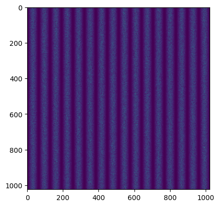
Create a sample function from a sinusoidal pattern
In [5]:
im_jax = jnp.tile(
    jnp.sin(np.arange(start=0, stop=16 * jnp.pi, step=jnp.pi / 64)), (1024, 1)
)
random_wave = jnp.asarray(random_image, dtype=jnp.complex128)
random_wave = random_wave / jnp.max(jnp.abs(random_wave))
sample_function = make_sample_function(im_jax, dx)
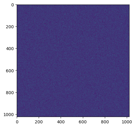
In [6]:
plt.imshow(jnp.abs(optical_wave.field) ** 2)
Out [6]:
<matplotlib.image.AxesImage at 0x7f91466268d0>
In [7]:
at_sample = linear_interaction(sample_function, optical_wave)
plt.imshow(jnp.abs(at_sample.field) ** 2)
Out [7]:
<matplotlib.image.AxesImage at 0x7f9146694740>
In [8]:
zoomed_wave = optical_zoom(at_sample, zoom_factor=9.7)
plt.imshow(jnp.abs(zoomed_wave.field) ** 2)
Out [8]:
<matplotlib.image.AxesImage at 0x7f9145d28a70>

Compare dx values.
As you can see using optical_zoom changes it.
In [9]:
zoomed_wave.dx, at_sample.dx, optical_wave.dx, sample_function.dx, dx
Out [9]:
(Array(0.00291, dtype=float64),
 Array(0.0003, dtype=float64),
 Array(0.0003, dtype=float64),
 Array(0.0003, dtype=float64),
 0.0003)
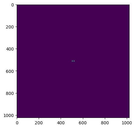
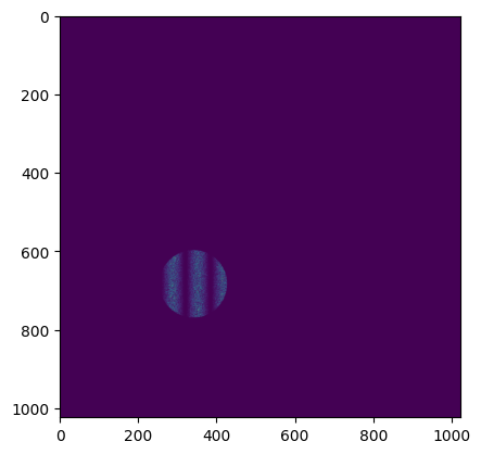
Use a circular aperture.
We can move the location of the aperture around too.
In [10]:
after_aperture = circular_aperture(
    zoomed_wave, diameter=0.5, center=jnp.array([-0.5, 0.5])
)
plt.imshow(jnp.abs(after_aperture.field) ** 2)
Out [10]:
<matplotlib.image.AxesImage at 0x7f9140b14590>

Propagate the beam
Use Fraunhofer propagation from fraunhofer_prop to propagate the beam. Other types available are Fresnel and Angular Spectrum Propagators.
In [17]:
at_camera_fraunhofer = jns.prop.fraunhofer_prop(after_aperture, 0.000001)
plt.imshow(jnp.abs(at_camera_fraunhofer.field) ** 2)
Out [17]:
<matplotlib.image.AxesImage at 0x7f90c0f84320>

In [18]:
at_camera_fraunhofer = jns.prop.fraunhofer_prop(after_aperture, 1)
plt.imshow(jnp.abs(at_camera_fraunhofer.field) ** 2)
Out [18]:
<matplotlib.image.AxesImage at 0x7f90bb172db0>
Use Fresnel propagation from fresnel_prop to propagate the beam now.
In [12]:
at_camera_fresnel = jns.prop.fresnel_prop(after_aperture, 1)
plt.imshow(jnp.abs(at_camera_fresnel.field) ** 2)
Out [12]:
<matplotlib.image.AxesImage at 0x7f913bfda4b0>
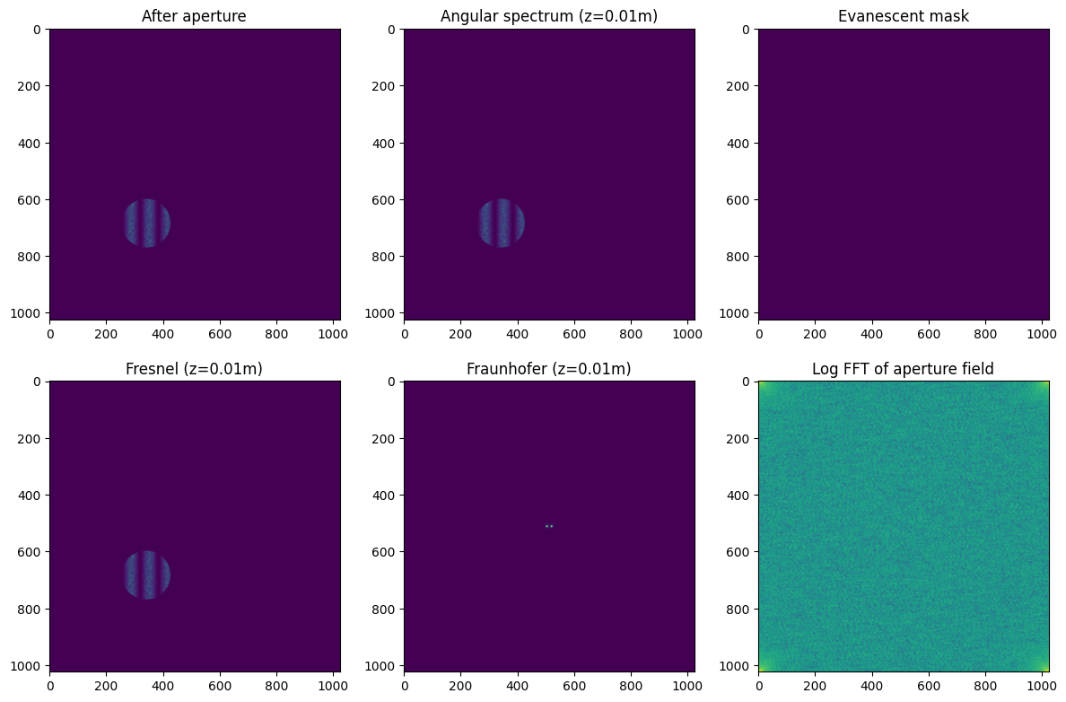
Use Angular Spectrum Propagation propagation from angular_spectrum_prop to propagate the beam now.
In [13]:
# Let's debug the angular spectrum propagation
print("After aperture field stats:")
print(f"  Wavelength: {after_aperture.wavelength}")
print(f"  dx (pixel size): {after_aperture.dx}")
print(f"  Field shape: {after_aperture.field.shape}")
print(
    f"  Field min/max magnitude: {jnp.abs(after_aperture.field).min():.6f}, {jnp.abs(after_aperture.field).max():.6f}"
)
print(f"  Non-zero elements: {(jnp.abs(after_aperture.field) > 0).sum()}")

# Try different distances
distances = [0.001, 0.01, 0.1, 1.0]
for z in distances:
    result = angular_spectrum_prop(after_aperture, z)
    print(f"\nAngular spectrum at z={z}m:")
    print(
        f"  Field min/max magnitude: {jnp.abs(result.field).min():.6f}, {jnp.abs(result.field).max():.6f}"
    )
    print(f"  Non-zero elements: {(jnp.abs(result.field) > 0).sum()}")

# Let's check the evanescent mask in angular spectrum
# Recreate what happens inside angular_spectrum_prop
z_test = 0.01
ny, nx = after_aperture.field.shape
wavenumber = 2 * jnp.pi / after_aperture.wavelength
fx = jnp.fft.fftfreq(nx, d=after_aperture.dx)
fy = jnp.fft.fftfreq(ny, d=after_aperture.dx)
fx_mesh, fy_mesh = jnp.meshgrid(fx, fy)
fsq_mesh = (fx_mesh**2) + (fy_mesh**2)
evanescent_mask = (1 / after_aperture.wavelength) ** 2 >= fsq_mesh

print(f"\nEvanescent mask analysis:")
print(f"  Total pixels: {evanescent_mask.size}")
print(f"  Pixels passing evanescent mask: {evanescent_mask.sum()}")
print(
    f"  Percentage passing: {100*evanescent_mask.sum()/evanescent_mask.size:.2f}%"
)
print(f"  Max spatial frequency squared: {fsq_mesh.max():.2e}")
print(f"  Wavelength cutoff squared: {(1/after_aperture.wavelength)**2:.2e}")

# Plot the results
fig, axes = plt.subplots(2, 3, figsize=(12, 8))
axes[0, 0].imshow(jnp.abs(after_aperture.field) ** 2)
axes[0, 0].set_title("After aperture")

at_camera_angular_spectrum = angular_spectrum_prop(after_aperture, 0.01)
axes[0, 1].imshow(jnp.abs(at_camera_angular_spectrum.field) ** 2)
axes[0, 1].set_title("Angular spectrum (z=0.01m)")

axes[0, 2].imshow(evanescent_mask.astype(float))
axes[0, 2].set_title("Evanescent mask")

# Compare with fresnel and fraunhofer at same distance
at_camera_fresnel_01 = fresnel_prop(after_aperture, 0.01)
axes[1, 0].imshow(jnp.abs(at_camera_fresnel_01.field) ** 2)
axes[1, 0].set_title("Fresnel (z=0.01m)")

at_camera_fraunhofer_01 = fraunhofer_prop(after_aperture, 0.01)
axes[1, 1].imshow(jnp.abs(at_camera_fraunhofer_01.field) ** 2)
axes[1, 1].set_title("Fraunhofer (z=0.01m)")

# Show FFT of aperture field
field_ft = jnp.fft.fft2(after_aperture.field)
axes[1, 2].imshow(jnp.log10(jnp.abs(field_ft) ** 2 + 1e-10))
axes[1, 2].set_title("Log FFT of aperture field")

plt.tight_layout()
plt.show()
After aperture field stats:
  Wavelength: 5.33e-07
  dx (pixel size): 0.0029099999999999994
  Field shape: (1024, 1024)
  Field min/max magnitude: 0.000000, 1.893390
  Non-zero elements: 23187

Angular spectrum at z=0.001m:
  Field min/max magnitude: 0.000000, 1.893390
  Non-zero elements: 1048576

Angular spectrum at z=0.01m:
  Field min/max magnitude: 0.000000, 1.893390
  Non-zero elements: 1048576

Angular spectrum at z=0.1m:
  Field min/max magnitude: 0.000000, 1.893389
  Non-zero elements: 1048576

Angular spectrum at z=1.0m:
  Field min/max magnitude: 0.000000, 1.893261
  Non-zero elements: 1048576

Evanescent mask analysis:
  Total pixels: 1048576
  Pixels passing evanescent mask: 1048576
  Percentage passing: 100.00%
  Max spatial frequency squared: 5.90e+04
  Wavelength cutoff squared: 3.52e+12
Propagator Comparison and Validity Regions
The three propagators have different validity regions based on the Fresnel number:
Angular Spectrum: Valid for all distances (most accurate, no approximations)
Fresnel: Valid when Fresnel number >> 1 (near-field)
Fraunhofer: Valid when Fresnel number << 1 (far-field)
The Fresnel number is: F = a²/(λz) where a is the aperture size, λ is wavelength, z is distance
In [14]:
# Calculate Fresnel numbers and compare propagators
aperture_diameter = 0.5  # meters (from circular_aperture call)
aperture_radius = aperture_diameter / 2

# After fixing wavelength, recalculate
wavelength_correct = 533e-9  # meters
distances_to_test = jnp.logspace(-3, 1, 20)  # From 1mm to 10m

print("Fresnel number analysis:")
print("-" * 60)
for z in distances_to_test:
    fresnel_number = aperture_radius**2 / (wavelength_correct * z)
    regime = (
        "Far-field (Fraunhofer)"
        if fresnel_number < 1
        else (
            "Near-field (Fresnel)"
            if fresnel_number < 10
            else "Very near-field"
        )
    )
    print(f"z = {z:.3f}m: F = {fresnel_number:.2f} - {regime}")

print("\n" + "=" * 60)
print("For aperture diameter = 0.5m and wavelength = 533nm:")
print("=" * 60)

# Critical distances
z_fresnel_transition = aperture_radius**2 / (10 * wavelength_correct)  # F = 10
z_fraunhofer_transition = aperture_radius**2 / wavelength_correct  # F = 1

print(
    f"\nFresnel approximation valid for: z << {z_fraunhofer_transition:.1f}m"
)
print(
    f"Fraunhofer approximation valid for: z >> {z_fraunhofer_transition:.1f}m"
)
print(f"Transition region: z ≈ {z_fraunhofer_transition:.1f}m")

# All three should give similar results in the Fraunhofer regime
print(
    f"\nAll propagators should give similar results when z > {10*z_fraunhofer_transition:.0f}m"
)
Fresnel number analysis:
------------------------------------------------------------
z = 0.001m: F = 117260787.99 - Very near-field
z = 0.002m: F = 72214846.51 - Very near-field
z = 0.003m: F = 44473384.04 - Very near-field
z = 0.004m: F = 27388854.00 - Very near-field
z = 0.007m: F = 16867376.74 - Very near-field
z = 0.011m: F = 10387743.79 - Very near-field
z = 0.018m: F = 6397273.43 - Very near-field
z = 0.030m: F = 3939749.40 - Very near-field
z = 0.048m: F = 2426287.62 - Very near-field
z = 0.078m: F = 1494224.89 - Very near-field
z = 0.127m: F = 920215.73 - Very near-field
z = 0.207m: F = 566713.21 - Very near-field
z = 0.336m: F = 349009.32 - Very near-field
z = 0.546m: F = 214936.76 - Very near-field
z = 0.886m: F = 132368.42 - Very near-field
z = 1.438m: F = 81518.86 - Very near-field
z = 2.336m: F = 50203.24 - Very near-field
z = 3.793m: F = 30917.58 - Very near-field
z = 6.158m: F = 19040.53 - Very near-field
z = 10.000m: F = 11726.08 - Very near-field

============================================================
For aperture diameter = 0.5m and wavelength = 533nm:
============================================================

Fresnel approximation valid for: z << 117260.8m
Fraunhofer approximation valid for: z >> 117260.8m
Transition region: z ≈ 117260.8m

All propagators should give similar results when z > 1172608m