Polarization in Wave Optics¶

This tutorial covers polarization representation and manipulation in Janssen.

Overview¶

Light is an electromagnetic wave with electric field oscillations. The polarization state describes the direction and temporal evolution of this oscillation:

Linear polarization: Electric field oscillates along a fixed direction
Circular polarization: Electric field rotates in a circle (right or left handed)
Elliptical polarization: General case with elliptical trajectory

This tutorial covers two complementary formalisms:

Jones calculus: For fully polarized, coherent light. Uses 2-component complex vectors and 2×2 matrices.
Mueller-Stokes calculus: For partially polarized or unpolarized light. Uses 4-component real vectors and 4×4 matrices.

Both are essential for different applications: Jones for coherent optical systems, Mueller-Stokes for depolarizing elements or incoherent sources.

In [1]:

import jax
import jax.numpy as jnp
import matplotlib.pyplot as plt
import matplotlib.gridspec as mpgs
from matplotlib.patches import Ellipse
import numpy as np
import janssen as jns
from janssen.models import (
    x_polarized_beam, y_polarized_beam, linear_polarized_beam,
    circular_polarized_beam, radially_polarized_beam, azimuthally_polarized_beam
)
from janssen.optics import polarizer_jones, waveplate_jones, quarter_waveplate, half_waveplate

# Configure matplotlib for publication figures
plt.rcParams['font.family'] = 'sans-serif'
plt.rcParams['font.sans-serif'] = ['TeX Gyre Heros']
plt.rcParams['mathtext.fontset'] = 'custom'
plt.rcParams['mathtext.rm'] = 'TeX Gyre Heros'
plt.rcParams['mathtext.it'] = 'TeX Gyre Heros:italic'
plt.rcParams['mathtext.bf'] = 'TeX Gyre Heros:bold'

plt.rcParams['font.size'] = 6
plt.rcParams['axes.titlesize'] = 7
plt.rcParams['axes.titleweight'] = 'bold'
plt.rcParams['axes.labelsize'] = 5
plt.rcParams['xtick.labelsize'] = 5
plt.rcParams['ytick.labelsize'] = 5
plt.rcParams['legend.fontsize'] = 6
plt.rcParams['figure.titlesize'] = 7

Setup: Physical Parameters¶

We define common parameters for our polarized beams.

In [2]:

# Physical parameters
wavelength = 633e-9  # HeNe laser, 633 nm
dx = 100e-9  # 100 nm pixel size
grid_size = (256, 256)
beam_radius = 10e-6  # 10 um beam radius

# Derived quantities
physical_size = grid_size[0] * dx
extent_um = [-physical_size/2*1e6, physical_size/2*1e6,
             -physical_size/2*1e6, physical_size/2*1e6]

print(f"Wavelength: {wavelength*1e9:.0f} nm")
print(f"Grid: {grid_size[0]}x{grid_size[1]}, dx = {dx*1e9:.0f} nm")
print(f"Beam radius: {beam_radius*1e6:.0f} um")
print(f"Physical extent: {physical_size*1e6:.1f} um")

Wavelength: 633 nm
Grid: 256x256, dx = 100 nm
Beam radius: 10 um
Physical extent: 25.6 um

Part I: Jones Calculus¶

1.1 Jones Vectors¶

A fully polarized monochromatic plane wave can be written as:

\[\begin{split}\vec{E}(z,t) = \begin{pmatrix} E_x \\ E_y \end{pmatrix} e^{i(kz - \omega t)}\end{split}\]

The Jones vector is the complex 2-component vector:

\[\begin{split}\vec{J} = \begin{pmatrix} E_x \\ E_y \end{pmatrix} = \begin{pmatrix} A_x e^{i\phi_x} \\ A_y e^{i\phi_y} \end{pmatrix}\end{split}\]

Common polarization states:

State	Jones Vector	Description
Horizontal (H)	\(\begin{pmatrix} 1 \\ 0 \end{pmatrix}\)	Linear along x
Vertical (V)	\(\begin{pmatrix} 0 \\ 1 \end{pmatrix}\)	Linear along y
Diagonal (+45°)	\(\frac{1}{\sqrt{2}}\begin{pmatrix} 1 \\ 1 \end{pmatrix}\)	Linear at 45°
Anti-diagonal (-45°)	\(\frac{1}{\sqrt{2}}\begin{pmatrix} 1 \\ -1 \end{pmatrix}\)	Linear at -45°
Right circular (RCP)	\(\frac{1}{\sqrt{2}}\begin{pmatrix} 1 \\ -i \end{pmatrix}\)	Clockwise rotation
Left circular (LCP)	\(\frac{1}{\sqrt{2}}\begin{pmatrix} 1 \\ i \end{pmatrix}\)	Counter-clockwise

In [3]:

# Create beams with different polarization states
beam_h = x_polarized_beam(wavelength, dx, grid_size, beam_radius=beam_radius)
beam_v = y_polarized_beam(wavelength, dx, grid_size, beam_radius=beam_radius)
beam_d = linear_polarized_beam(wavelength, dx, grid_size,
                                polarization_angle=jnp.pi/4, beam_radius=beam_radius)
beam_rcp = circular_polarized_beam(wavelength, dx, grid_size,
                                    handedness='right', beam_radius=beam_radius)
beam_lcp = circular_polarized_beam(wavelength, dx, grid_size,
                                    handedness='left', beam_radius=beam_radius)

# Extract Jones vectors at beam center
center = grid_size[0] // 2

def get_jones_at_center(beam):
    """Extract normalized Jones vector at beam center."""
    j = beam.field[center, center, :]
    return j / jnp.abs(j[0])  # Normalize to Ex = 1

print("Jones vectors at beam center (normalized to Ex=1):")
print(f"H-polarized:   [{beam_h.field[center,center,0]:.3f}, {beam_h.field[center,center,1]:.3f}]")
print(f"V-polarized:   [{beam_v.field[center,center,0]:.3f}, {beam_v.field[center,center,1]:.3f}]")
j_d = get_jones_at_center(beam_d)
print(f"+45° linear:   [{j_d[0]:.3f}, {j_d[1]:.3f}]")
j_rcp = get_jones_at_center(beam_rcp)
print(f"RCP:           [{j_rcp[0]:.3f}, {j_rcp[1]:.3f}]")
j_lcp = get_jones_at_center(beam_lcp)
print(f"LCP:           [{j_lcp[0]:.3f}, {j_lcp[1]:.3f}]")

WARNING:2026-01-05 01:54:30,190:jax._src.xla_bridge:864: An NVIDIA GPU may be present on this machine, but a CUDA-enabled jaxlib is not installed. Falling back to cpu.

Jones vectors at beam center (normalized to Ex=1):
H-polarized:   [1.000+0.000j, 0.000+0.000j]
V-polarized:   [0.000+0.000j, 1.000+0.000j]
+45° linear:   [1.000+0.000j, 1.000+0.000j]
RCP:           [1.000+0.000j, 0.000-1.000j]
LCP:           [1.000+0.000j, 0.000+1.000j]

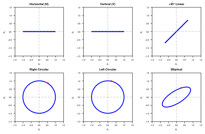
1.2 Visualizing Polarization States¶

We visualize the electric field components and polarization ellipses for each state.

In [4]:

def compute_polarization_ellipse(Ex, Ey):
    """Compute polarization ellipse parameters from Jones vector components.

    Parameters
    ----------
    Ex, Ey : complex
        Jones vector components

    Returns
    -------
    dict with keys:
        'a': semi-major axis
        'b': semi-minor axis
        'theta': orientation angle (radians)
        'handedness': 'right', 'left', or 'linear'
        'ellipticity': b/a (0 for linear, 1 for circular)
    """
    # Amplitudes and phases
    ax, ay = jnp.abs(Ex), jnp.abs(Ey)
    phi_x, phi_y = jnp.angle(Ex), jnp.angle(Ey)
    delta = phi_y - phi_x  # Phase difference

    # Polarization ellipse parameters (Born & Wolf)
    # tan(2*psi) = tan(2*alpha) * cos(delta)
    # sin(2*chi) = sin(2*alpha) * sin(delta)
    # where alpha = arctan(ay/ax), psi = orientation, chi = ellipticity angle

    alpha = jnp.arctan2(ay, ax)

    # Orientation angle psi
    cos_delta = jnp.cos(delta)
    tan_2alpha = jnp.tan(2 * alpha)
    psi = 0.5 * jnp.arctan2(tan_2alpha * cos_delta, 1.0)

    # Ellipticity angle chi
    sin_delta = jnp.sin(delta)
    sin_2alpha = jnp.sin(2 * alpha)
    sin_2chi = sin_2alpha * sin_delta
    sin_2chi = jnp.clip(sin_2chi, -1, 1)
    chi = 0.5 * jnp.arcsin(sin_2chi)

    # Semi-axes from total intensity
    I_total = ax**2 + ay**2
    a = jnp.sqrt(I_total) * jnp.abs(jnp.cos(chi))
    b = jnp.sqrt(I_total) * jnp.abs(jnp.sin(chi))

    # Ensure a >= b
    a, b = jnp.maximum(a, b), jnp.minimum(a, b)

    # Handedness: sin(delta) > 0 -> left, < 0 -> right
    if jnp.abs(sin_delta) < 0.01:
        handedness = 'linear'
    elif sin_delta > 0:
        handedness = 'left'
    else:
        handedness = 'right'

    ellipticity = float(b / (a + 1e-10))

    return {
        'a': float(a),
        'b': float(b),
        'theta': float(psi),
        'handedness': handedness,
        'ellipticity': ellipticity
    }

In [5]:

def plot_polarization_state(ax, Ex, Ey, title):
    """Plot polarization ellipse for a Jones vector."""
    params = compute_polarization_ellipse(Ex, Ey)

    # Normalize for visualization
    scale = 1.0 / max(params['a'], 0.01)
    a_norm = params['a'] * scale
    b_norm = params['b'] * scale

    # Draw ellipse
    ellipse = Ellipse((0, 0), 2*a_norm, 2*b_norm,
                       angle=np.degrees(params['theta']),
                       fill=False, color='blue', linewidth=2)
    ax.add_patch(ellipse)

    # Draw arrow showing rotation direction for circular/elliptical
    if params['handedness'] != 'linear':
        # Draw small arrow on ellipse
        t = np.pi/4  # Position on ellipse
        x_arrow = a_norm * np.cos(t) * np.cos(params['theta']) - b_norm * np.sin(t) * np.sin(params['theta'])
        y_arrow = a_norm * np.cos(t) * np.sin(params['theta']) + b_norm * np.sin(t) * np.cos(params['theta'])

        # Tangent direction
        dx = -a_norm * np.sin(t) * np.cos(params['theta']) - b_norm * np.cos(t) * np.sin(params['theta'])
        dy = -a_norm * np.sin(t) * np.sin(params['theta']) + b_norm * np.cos(t) * np.cos(params['theta'])

        if params['handedness'] == 'right':
            dx, dy = -dx, -dy

        # Normalize and scale arrow
        norm = np.sqrt(dx**2 + dy**2)
        dx, dy = 0.3 * dx/norm, 0.3 * dy/norm

        ax.annotate('', xy=(x_arrow+dx, y_arrow+dy), xytext=(x_arrow, y_arrow),
                    arrowprops=dict(arrowstyle='->', color='red', lw=1.5))

    ax.set_xlim(-1.5, 1.5)
    ax.set_ylim(-1.5, 1.5)
    ax.set_aspect('equal')
    ax.axhline(y=0, color='gray', linestyle='--', alpha=0.3)
    ax.axvline(x=0, color='gray', linestyle='--', alpha=0.3)
    ax.set_xlabel('$E_x$')
    ax.set_ylabel('$E_y$')
    ax.set_title(title)

# Plot all polarization states
fig, axes = plt.subplots(2, 3, figsize=(7, 4.5))

states = [
    (1+0j, 0+0j, 'Horizontal (H)'),
    (0+0j, 1+0j, 'Vertical (V)'),
    (1+0j, 1+0j, '+45° Linear'),
    (1+0j, -1j, 'Right Circular'),
    (1+0j, 1j, 'Left Circular'),
    (1+0j, 0.5+0.5j, 'Elliptical')
]

for ax, (Ex, Ey, title) in zip(axes.flat, states):
    # Normalize
    norm = np.sqrt(abs(Ex)**2 + abs(Ey)**2)
    plot_polarization_state(ax, Ex/norm, Ey/norm, title)

plt.tight_layout()
plt.savefig('Figures/polarization_jones_states.pdf', bbox_inches='tight')
plt.savefig('Figures/polarization_jones_states.png', dpi=300, bbox_inches='tight')
plt.show()

../_images/tutorials_Polarization_8_0.png

1.3 Jones Matrices¶

Optical elements that transform polarization are represented by 2×2 Jones matrices:

\[\vec{J}_{out} = \mathbf{M} \cdot \vec{J}_{in}\]

Common Jones matrices:

Linear Polarizer at angle θ:¶

\[\begin{split}\mathbf{P}(\theta) = \begin{pmatrix} \cos^2\theta & \cos\theta\sin\theta \\ \cos\theta\sin\theta & \sin^2\theta \end{pmatrix}\end{split}\]

Waveplate with retardance δ and fast axis at angle θ:¶

\[\begin{split}\mathbf{W}(\delta, \theta) = \mathbf{R}(-\theta) \begin{pmatrix} 1 & 0 \\ 0 & e^{i\delta} \end{pmatrix} \mathbf{R}(\theta)\end{split}\]

Special cases:

Quarter-wave plate (QWP): \(\delta = \pi/2\) — converts linear to circular
Half-wave plate (HWP): \(\delta = \pi\) — rotates linear polarization by \(2\theta\)

In [6]:

# Demonstrate Jones matrices with Janssen functions

# Start with x-polarized beam
beam_x = x_polarized_beam(wavelength, dx, grid_size, beam_radius=beam_radius)
print("Initial: X-polarized beam")
print(f"  Jones at center: [{beam_x.field[center,center,0]:.3f}, {beam_x.field[center,center,1]:.3f}]")

# Pass through horizontal polarizer (should pass unchanged)
beam_after_pol_h = polarizer_jones(beam_x, theta=0.0)
print("\nAfter horizontal polarizer (θ=0):")
print(f"  Jones at center: [{beam_after_pol_h.field[center,center,0]:.3f}, {beam_after_pol_h.field[center,center,1]:.3f}]")

# Pass through vertical polarizer (should block)
beam_after_pol_v = polarizer_jones(beam_x, theta=jnp.pi/2)
print("\nAfter vertical polarizer (θ=π/2):")
print(f"  Jones at center: [{beam_after_pol_v.field[center,center,0]:.3f}, {beam_after_pol_v.field[center,center,1]:.3f}]")
print(f"  (Blocked! Intensity = {jnp.abs(beam_after_pol_v.field[center,center,0])**2 + jnp.abs(beam_after_pol_v.field[center,center,1])**2:.6f})")

# Pass through 45° polarizer
beam_after_pol_45 = polarizer_jones(beam_x, theta=jnp.pi/4)
j45 = beam_after_pol_45.field[center,center,:]
print("\nAfter 45° polarizer (θ=π/4):")
print(f"  Jones at center: [{j45[0]:.3f}, {j45[1]:.3f}]")
print(f"  Ratio Ey/Ex = {j45[1]/j45[0]:.3f} (should be 1.0)")

Initial: X-polarized beam
  Jones at center: [1.000+0.000j, 0.000+0.000j]

After horizontal polarizer (θ=0):
  Jones at center: [1.000+0.000j, 0.000+0.000j]

After vertical polarizer (θ=π/2):
  Jones at center: [0.000+0.000j, 0.000+0.000j]
  (Blocked! Intensity = 0.000000)

After 45° polarizer (θ=π/4):
  Jones at center: [0.500+0.000j, 0.500+0.000j]
  Ratio Ey/Ex = 1.000+0.000j (should be 1.0)

In [7]:

# Demonstrate waveplates

# Start with +45° linear polarization
beam_45 = linear_polarized_beam(wavelength, dx, grid_size,
                                 polarization_angle=jnp.pi/4, beam_radius=beam_radius)
j_in = beam_45.field[center,center,:]
print("Initial: +45° linear polarization")
print(f"  Jones: [{j_in[0]:.3f}, {j_in[1]:.3f}]")

# Quarter-wave plate with fast axis horizontal -> converts to circular
beam_after_qwp = quarter_waveplate(beam_45, theta=0.0)
j_qwp = beam_after_qwp.field[center,center,:]
print("\nAfter QWP (fast axis horizontal):")
print(f"  Jones: [{j_qwp[0]:.3f}, {j_qwp[1]:.3f}]")
print(f"  Phase difference: {jnp.angle(j_qwp[1]) - jnp.angle(j_qwp[0]):.3f} rad")
print(f"  (Should be π/2 = {jnp.pi/2:.3f} for circular polarization)")

# Start with x-polarized
beam_x = x_polarized_beam(wavelength, dx, grid_size, beam_radius=beam_radius)

# Half-wave plate at 22.5° rotates polarization by 45°
beam_after_hwp = half_waveplate(beam_x, theta=jnp.pi/8)  # 22.5°
j_hwp = beam_after_hwp.field[center,center,:]
print("\nX-polarized after HWP at 22.5°:")
print(f"  Jones: [{j_hwp[0]:.3f}, {j_hwp[1]:.3f}]")
pol_angle = jnp.arctan2(jnp.abs(j_hwp[1]), jnp.abs(j_hwp[0]))
print(f"  Polarization angle: {jnp.degrees(pol_angle):.1f}° (should be 45°)")

Initial: +45° linear polarization
  Jones: [0.707+0.000j, 0.707+0.000j]

After QWP (fast axis horizontal):
  Jones: [0.707+0.000j, 0.000+0.707j]
  Phase difference: 1.571 rad
  (Should be π/2 = 1.571 for circular polarization)

X-polarized after HWP at 22.5°:
  Jones: [0.707+0.000j, 0.707-0.000j]
  Polarization angle: 45.0° (should be 45°)

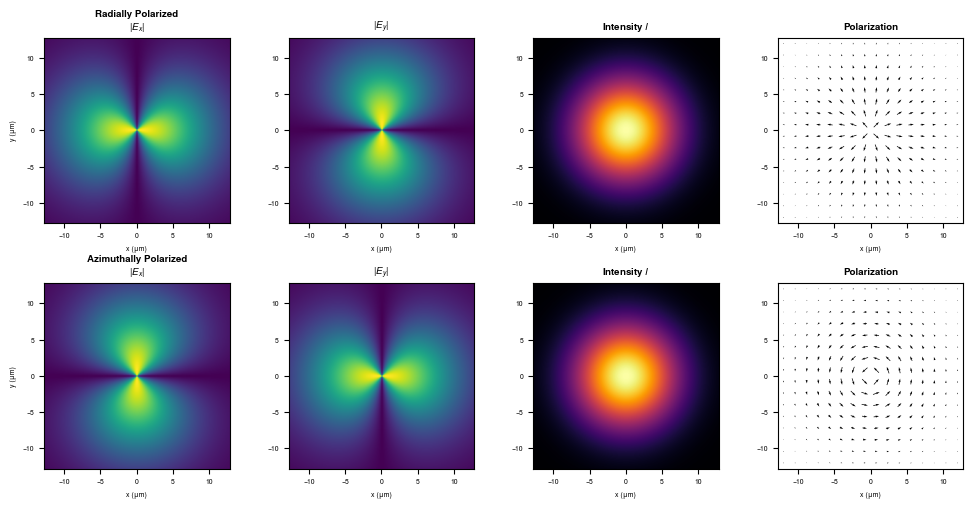
1.4 Cylindrical Vector Beams¶

Unlike uniformly polarized beams, cylindrical vector beams have spatially varying polarization:

Radially polarized: \(\vec{E} \propto \hat{r}\) (points outward from axis)
Azimuthally polarized: \(\vec{E} \propto \hat{\phi}\) (tangent to circles)

These beams have unique focusing properties crucial for high-NA microscopy.

In [8]:

def plot_polarized_beam(wf, title, ax_row):
    """Plot a polarized beam: |Ex|, |Ey|, total intensity, and polarization vectors."""
    ex = wf.field[..., 0]
    ey = wf.field[..., 1]

    # |Ex|
    ax_row[0].imshow(jnp.abs(ex), cmap='viridis', extent=extent_um)
    ax_row[0].set_title(f'{title}\n$|E_x|$')
    ax_row[0].set_xlabel('x (μm)')
    ax_row[0].set_ylabel('y (μm)')

    # |Ey|
    ax_row[1].imshow(jnp.abs(ey), cmap='viridis', extent=extent_um)
    ax_row[1].set_title('$|E_y|$')
    ax_row[1].set_xlabel('x (μm)')

    # Total intensity
    I_total = jnp.abs(ex)**2 + jnp.abs(ey)**2
    ax_row[2].imshow(I_total, cmap='inferno', extent=extent_um)
    ax_row[2].set_title('Intensity $I$')
    ax_row[2].set_xlabel('x (μm)')

    # Polarization vectors (quiver plot)
    ny, nx = ex.shape
    step = 16
    y_idx, x_idx = jnp.mgrid[step//2:ny:step, step//2:nx:step]

    # Physical coordinates
    x_coords = (x_idx - nx/2) * dx * 1e6
    y_coords = (y_idx - ny/2) * dx * 1e6

    u = jnp.real(ex[y_idx, x_idx])
    v = jnp.real(ey[y_idx, x_idx])

    ax_row[3].quiver(x_coords, y_coords, u, v, pivot='mid', scale=25)
    ax_row[3].set_xlim(extent_um[0], extent_um[1])
    ax_row[3].set_ylim(extent_um[2], extent_um[3])
    ax_row[3].set_aspect('equal')
    ax_row[3].set_title('Polarization')
    ax_row[3].set_xlabel('x (μm)')

# Create cylindrical vector beams
radial = radially_polarized_beam(wavelength, dx, grid_size, beam_radius=beam_radius)
azimuthal = azimuthally_polarized_beam(wavelength, dx, grid_size, beam_radius=beam_radius)

# Plot
fig, axes = plt.subplots(2, 4, figsize=(10, 5))
plot_polarized_beam(radial, 'Radially Polarized', axes[0])
plot_polarized_beam(azimuthal, 'Azimuthally Polarized', axes[1])

plt.tight_layout()
plt.savefig('Figures/polarization_cvb.pdf', bbox_inches='tight')
plt.savefig('Figures/polarization_cvb.png', dpi=300, bbox_inches='tight')
plt.show()

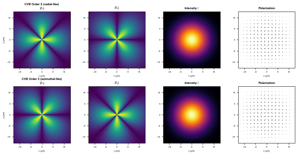
../_images/tutorials_Polarization_13_0.png

1.5 Generalized Cylindrical Vector Beams¶

Higher-order cylindrical vector beams have multiple polarization singularities. The order parameter controls the number of rotations of the polarization direction around the beam axis.

For order \(m\):

\(m = 1\): Standard radial/azimuthal beams
\(m = 2\): Four-fold symmetric polarization pattern
\(m = 3\): Six-fold symmetric pattern

The phase_offset parameter interpolates between radial-like (\(\phi_0 = 0\)) and azimuthal-like (\(\phi_0 = \pi/2\)) patterns.

In [9]:

from janssen.models import generalized_cylindrical_vector_beam

# Higher-order CVB (order 2)
cvb_order2_radial = generalized_cylindrical_vector_beam(
    wavelength=wavelength,
    dx=dx,
    grid_size=grid_size,
    order=2,
    phase_offset=0.0,  # Radial-like
    beam_radius=beam_radius,
)

cvb_order2_azim = generalized_cylindrical_vector_beam(
    wavelength=wavelength,
    dx=dx,
    grid_size=grid_size,
    order=2,
    phase_offset=jnp.pi/2,  # Azimuthal-like
    beam_radius=beam_radius,
)

# Plot comparison
fig, axes = plt.subplots(2, 4, figsize=(10, 5))
plot_polarized_beam(cvb_order2_radial, 'CVB Order 2 (radial-like)', axes[0])
plot_polarized_beam(cvb_order2_azim, 'CVB Order 2 (azimuthal-like)', axes[1])

plt.tight_layout()
plt.savefig('Figures/polarization_cvb_order2.pdf', bbox_inches='tight')
plt.savefig('Figures/polarization_cvb_order2.png', dpi=300, bbox_inches='tight')
plt.show()

../_images/tutorials_Polarization_15_0.png

Part II: Mueller-Stokes Calculus¶

2.1 Stokes Parameters¶

For partially polarized or unpolarized light, Jones calculus is insufficient. The Stokes vector provides a complete description using four real, measurable quantities:

\[\begin{split}\vec{S} = \begin{pmatrix} S_0 \\ S_1 \\ S_2 \\ S_3 \end{pmatrix} = \begin{pmatrix} I \\ I_H - I_V \\ I_{+45} - I_{-45} \\ I_{RCP} - I_{LCP} \end{pmatrix}\end{split}\]

where:

\(S_0 = I\): Total intensity
\(S_1\): Preference for horizontal vs vertical polarization
\(S_2\): Preference for +45° vs -45° polarization
\(S_3\): Preference for right vs left circular polarization

The degree of polarization (DOP):

\[P = \frac{\sqrt{S_1^2 + S_2^2 + S_3^2}}{S_0}\]

\(P = 1\): Fully polarized
\(P = 0\): Unpolarized
\(0 < P < 1\): Partially polarized

In [10]:

def jones_to_stokes(Ex, Ey):
    """Convert Jones vector to Stokes parameters.

    For fully polarized light, computes Stokes vector from Jones vector.

    Parameters
    ----------
    Ex, Ey : complex
        Jones vector components

    Returns
    -------
    S : array of shape (4,)
        Stokes vector [S0, S1, S2, S3]
    """
    S0 = jnp.abs(Ex)**2 + jnp.abs(Ey)**2
    S1 = jnp.abs(Ex)**2 - jnp.abs(Ey)**2
    S2 = 2 * jnp.real(Ex * jnp.conj(Ey))
    S3 = 2 * jnp.imag(Ex * jnp.conj(Ey))

    return jnp.array([S0, S1, S2, S3])

def degree_of_polarization(S):
    """Compute degree of polarization from Stokes vector."""
    return jnp.sqrt(S[1]**2 + S[2]**2 + S[3]**2) / (S[0] + 1e-10)

def stokes_to_jones(S):
    """Convert Stokes vector to Jones vector (for fully polarized light).

    Note: Only valid for DOP = 1. Returns one possible Jones vector
    (the global phase is arbitrary).
    """
    S0, S1, S2, S3 = S

    # Amplitude
    ax = jnp.sqrt((S0 + S1) / 2)
    ay = jnp.sqrt((S0 - S1) / 2)

    # Phase difference
    delta = jnp.arctan2(S3, S2)

    Ex = ax
    Ey = ay * jnp.exp(1j * delta)

    return Ex, Ey

In [11]:

# Compute Stokes parameters for various polarization states
print("Stokes parameters for common polarization states:")
print("State               S0    S1    S2    S3    DOP")
print("-" * 55)

states = [
    (1+0j, 0+0j, 'Horizontal'),
    (0+0j, 1+0j, 'Vertical'),
    (1/jnp.sqrt(2), 1/jnp.sqrt(2), '+45°'),
    (1/jnp.sqrt(2), -1/jnp.sqrt(2), '-45°'),
    (1/jnp.sqrt(2), -1j/jnp.sqrt(2), 'RCP'),
    (1/jnp.sqrt(2), 1j/jnp.sqrt(2), 'LCP'),
]

for Ex, Ey, name in states:
    S = jones_to_stokes(Ex, Ey)
    dop = degree_of_polarization(S)
    print(f"{name:18s}  {S[0]:5.2f} {S[1]:5.2f} {S[2]:5.2f} {S[3]:5.2f}  {dop:.2f}")

Stokes parameters for common polarization states:
State               S0    S1    S2    S3    DOP
-------------------------------------------------------
Horizontal           1.00  1.00  0.00  0.00  1.00
Vertical             1.00 -1.00  0.00  0.00  1.00
+45°                 1.00  0.00  1.00  0.00  1.00
-45°                 1.00  0.00 -1.00  0.00  1.00
RCP                  1.00  0.00 -0.00  1.00  1.00
LCP                  1.00  0.00  0.00 -1.00  1.00

2.2 Mueller Matrices¶

Optical elements transform Stokes vectors via 4×4 Mueller matrices:

\[\vec{S}_{out} = \mathbf{M} \cdot \vec{S}_{in}\]

Mueller matrices can describe:

Polarizing elements (same as Jones)
Depolarizing elements (cannot be described by Jones!)
Partially polarizing elements

Linear Polarizer (horizontal):¶

\[\begin{split}\mathbf{M}_{H} = \frac{1}{2}\begin{pmatrix} 1 & 1 & 0 & 0 \\ 1 & 1 & 0 & 0 \\ 0 & 0 & 0 & 0 \\ 0 & 0 & 0 & 0 \end{pmatrix}\end{split}\]

Quarter-wave plate (fast axis horizontal):¶

\[\begin{split}\mathbf{M}_{QWP} = \begin{pmatrix} 1 & 0 & 0 & 0 \\ 0 & 1 & 0 & 0 \\ 0 & 0 & 0 & 1 \\ 0 & 0 & -1 & 0 \end{pmatrix}\end{split}\]

Ideal Depolarizer:¶

\[\begin{split}\mathbf{M}_{depol} = \begin{pmatrix} 1 & 0 & 0 & 0 \\ 0 & 0 & 0 & 0 \\ 0 & 0 & 0 & 0 \\ 0 & 0 & 0 & 0 \end{pmatrix}\end{split}\]

In [12]:

def mueller_linear_polarizer(theta):
    """Mueller matrix for linear polarizer at angle theta."""
    c2 = jnp.cos(2*theta)
    s2 = jnp.sin(2*theta)

    M = 0.5 * jnp.array([
        [1,    c2,   s2,   0],
        [c2,   c2**2, c2*s2, 0],
        [s2,   c2*s2, s2**2, 0],
        [0,    0,    0,    0]
    ])
    return M

def mueller_waveplate(delta, theta):
    """Mueller matrix for waveplate with retardance delta, fast axis at theta."""
    c2 = jnp.cos(2*theta)
    s2 = jnp.sin(2*theta)
    cd = jnp.cos(delta)
    sd = jnp.sin(delta)

    M = jnp.array([
        [1, 0, 0, 0],
        [0, c2**2 + s2**2*cd, c2*s2*(1-cd), -s2*sd],
        [0, c2*s2*(1-cd), s2**2 + c2**2*cd, c2*sd],
        [0, s2*sd, -c2*sd, cd]
    ])
    return M

def mueller_qwp(theta):
    """Mueller matrix for quarter-wave plate."""
    return mueller_waveplate(jnp.pi/2, theta)

def mueller_hwp(theta):
    """Mueller matrix for half-wave plate."""
    return mueller_waveplate(jnp.pi, theta)

def mueller_depolarizer(p=0.0):
    """Mueller matrix for partial depolarizer.

    p = 0: complete depolarization
    p = 1: no depolarization (identity)
    """
    return jnp.array([
        [1, 0, 0, 0],
        [0, p, 0, 0],
        [0, 0, p, 0],
        [0, 0, 0, p]
    ])

def apply_mueller(M, S):
    """Apply Mueller matrix to Stokes vector."""
    return M @ S

In [13]:

# Demonstrate Mueller calculus

# Start with unpolarized light
S_unpol = jnp.array([1.0, 0.0, 0.0, 0.0])
print("Unpolarized light:")
print(f"  Stokes: {S_unpol}")
print(f"  DOP: {degree_of_polarization(S_unpol):.2f}")

# Pass through horizontal polarizer
M_H = mueller_linear_polarizer(0.0)
S_after_pol = apply_mueller(M_H, S_unpol)
print("\nAfter horizontal polarizer:")
print(f"  Stokes: {S_after_pol}")
print(f"  DOP: {degree_of_polarization(S_after_pol):.2f}")

# Start with H-polarized, pass through QWP at 45°
S_H = jnp.array([1.0, 1.0, 0.0, 0.0])
M_QWP = mueller_qwp(jnp.pi/4)  # Fast axis at 45°
S_after_qwp = apply_mueller(M_QWP, S_H)
print("\nH-polarized through QWP at 45°:")
print(f"  Input Stokes:  {S_H}")
print(f"  Output Stokes: {S_after_qwp}")
print(f"  (Should be circularly polarized: S3 ≠ 0)")

# Demonstrate depolarization (impossible with Jones!)
S_polarized = jnp.array([1.0, 0.5, 0.5, 0.5])  # Elliptically polarized
print(f"\nElliptically polarized (DOP = {degree_of_polarization(S_polarized):.2f}):")
print(f"  Stokes: {S_polarized}")

# Partial depolarization
for p in [0.8, 0.5, 0.0]:
    M_dep = mueller_depolarizer(p)
    S_out = apply_mueller(M_dep, S_polarized)
    print(f"  After depolarizer (p={p}): DOP = {degree_of_polarization(S_out):.2f}")

Unpolarized light:
  Stokes: [1. 0. 0. 0.]
  DOP: 0.00

After horizontal polarizer:
  Stokes: [0.5 0.5 0.  0. ]
  DOP: 1.00

H-polarized through QWP at 45°:
  Input Stokes:  [1. 1. 0. 0.]
  Output Stokes: [1.000000e+00 6.123234e-17 6.123234e-17 1.000000e+00]
  (Should be circularly polarized: S3 ≠ 0)

Elliptically polarized (DOP = 0.87):
  Stokes: [1.  0.5 0.5 0.5]
  After depolarizer (p=0.8): DOP = 0.69
  After depolarizer (p=0.5): DOP = 0.43
  After depolarizer (p=0.0): DOP = 0.00

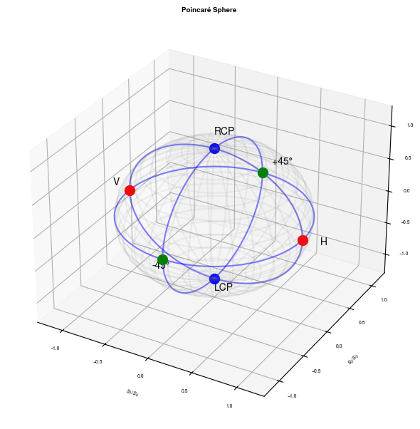
2.3 The Poincaré Sphere¶

Fully polarized states can be visualized on the Poincaré sphere, where:

Coordinates \((S_1/S_0, S_2/S_0, S_3/S_0)\) define a point on the unit sphere
Equator: linear polarization (H, V, ±45°)
Poles: circular polarization (RCP at north, LCP at south)
Interior points: partially polarized (DOP < 1)
Origin: unpolarized

In [14]:

from mpl_toolkits.mplot3d import Axes3D

fig = plt.figure(figsize=(7, 6))
ax = fig.add_subplot(111, projection='3d')

# Draw sphere wireframe
u = np.linspace(0, 2*np.pi, 30)
v = np.linspace(0, np.pi, 20)
x_sphere = np.outer(np.cos(u), np.sin(v))
y_sphere = np.outer(np.sin(u), np.sin(v))
z_sphere = np.outer(np.ones(np.size(u)), np.cos(v))
ax.plot_wireframe(x_sphere, y_sphere, z_sphere, alpha=0.1, color='gray')

# Draw equator and meridians
theta = np.linspace(0, 2*np.pi, 100)
ax.plot(np.cos(theta), np.sin(theta), np.zeros_like(theta), 'b-', alpha=0.5)
ax.plot(np.zeros_like(theta), np.cos(theta), np.sin(theta), 'b-', alpha=0.5)
ax.plot(np.cos(theta), np.zeros_like(theta), np.sin(theta), 'b-', alpha=0.5)

# Plot key polarization states
states_3d = [
    ([1, 0, 0], 'H', 'red'),
    ([-1, 0, 0], 'V', 'red'),
    ([0, 1, 0], '+45°', 'green'),
    ([0, -1, 0], '-45°', 'green'),
    ([0, 0, 1], 'RCP', 'blue'),
    ([0, 0, -1], 'LCP', 'blue'),
]

for coords, label, color in states_3d:
    ax.scatter(*coords, s=100, c=color, marker='o')
    ax.text(coords[0]*1.2, coords[1]*1.2, coords[2]*1.2, label, fontsize=10)

# Draw path: H -> QWP -> circular
# QWP at 45° rotates around S1 axis by 90°
t_path = np.linspace(0, np.pi/2, 50)
path_x = np.ones_like(t_path)  # Stay at S1 = 1
path_y = np.zeros_like(t_path)
path_z = np.sin(t_path)  # Go from 0 to 1
# Actually for QWP at 0° on +45° input:
path_x = np.cos(t_path)  # S1 stays
path_y = np.sin(t_path) * np.cos(t_path)  # S2 changes
path_z = np.sin(t_path)  # S3 changes

ax.set_xlabel('$S_1/S_0$')
ax.set_ylabel('$S_2/S_0$')
ax.set_zlabel('$S_3/S_0$')
ax.set_title('Poincaré Sphere')

# Equal aspect ratio
ax.set_xlim(-1.3, 1.3)
ax.set_ylim(-1.3, 1.3)
ax.set_zlim(-1.3, 1.3)

plt.tight_layout()
plt.savefig('Figures/polarization_poincare.pdf', bbox_inches='tight')
plt.savefig('Figures/polarization_poincare.png', dpi=300, bbox_inches='tight')
plt.show()

../_images/tutorials_Polarization_23_0.png

Part III: Differentiable Polarization Optics¶

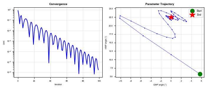
3.1 Gradient-Based Optimization¶

Because Janssen implements polarization using JAX, we can compute gradients with respect to polarization parameters. This enables:

Polarimeter inversion: Recover waveplate angles from measured intensities
Polarization state optimization: Find optical elements to achieve target polarization
Sensitivity analysis: How does output depend on element orientation errors?

In [15]:

# Problem: Given H-polarized input and a target output polarization,
# find the QWP and HWP angles to achieve it.

# Target: +45° linear polarization
target_jones = jnp.array([1.0, 1.0]) / jnp.sqrt(2)

def optical_system(qwp_angle, hwp_angle):
    """H-polarized beam through QWP then HWP. Returns output Jones vector."""
    # Start with H-polarized
    beam = x_polarized_beam(wavelength, dx, grid_size, beam_radius=beam_radius)

    # Apply QWP
    beam = quarter_waveplate(beam, theta=qwp_angle)

    # Apply HWP
    beam = half_waveplate(beam, theta=hwp_angle)

    # Return Jones vector at center
    return beam.field[center, center, :]

def loss_fn(params):
    """MSE between output and target Jones vectors."""
    qwp_angle, hwp_angle = params
    output = optical_system(qwp_angle, hwp_angle)

    # Normalize both for comparison (ignore global phase)
    output_norm = output / jnp.abs(output[0])
    target_norm = target_jones / jnp.abs(target_jones[0])

    # Match magnitudes and relative phase
    return jnp.sum(jnp.abs(output_norm - target_norm)**2)

# Test the loss function
test_params = jnp.array([0.0, 0.0])
print(f"Loss at (0, 0): {loss_fn(test_params):.4f}")

# Compute gradient
grad_fn = jax.grad(loss_fn)
grads = grad_fn(test_params)
print(f"Gradient: {grads}")

Loss at (0, 0): 1.0000
Gradient: [ 2. -4.]

In [16]:

import optax

# Optimize to find waveplate angles
optimizer = optax.adam(learning_rate=0.1)

# Initial guess
params = jnp.array([0.1, 0.1])  # Small random angles
opt_state = optimizer.init(params)

n_iterations = 100
loss_history = []
params_history = [params.copy()]

print("Optimizing QWP and HWP angles to achieve +45° polarization...")
print(f"Target Jones: {target_jones}")
print(f"\nInitial params: QWP={jnp.degrees(params[0]):.1f}°, HWP={jnp.degrees(params[1]):.1f}°")

for i in range(n_iterations):
    loss = loss_fn(params)
    loss_history.append(float(loss))

    grads = grad_fn(params)
    updates, opt_state = optimizer.update(grads, opt_state)
    params = optax.apply_updates(params, updates)
    params_history.append(params.copy())

    if (i+1) % 20 == 0:
        output = optical_system(params[0], params[1])
        print(f"Iter {i+1}: loss={loss:.6f}, QWP={jnp.degrees(params[0]):.1f}°, HWP={jnp.degrees(params[1]):.1f}°")

# Final result
final_output = optical_system(params[0], params[1])
final_output_norm = final_output / jnp.abs(final_output[0])
print(f"\nFinal params: QWP={jnp.degrees(params[0]):.1f}°, HWP={jnp.degrees(params[1]):.1f}°")
print(f"Output Jones: [{final_output_norm[0]:.3f}, {final_output_norm[1]:.3f}]")
print(f"Target Jones: [{target_jones[0]/target_jones[0]:.3f}, {target_jones[1]/target_jones[0]:.3f}]")

Optimizing QWP and HWP angles to achieve +45° polarization...
Target Jones: [0.70710678 0.70710678]

Initial params: QWP=5.7°, HWP=5.7°
Iter 20: loss=0.000471, QWP=1.5°, HWP=22.1°
Iter 40: loss=0.002001, QWP=-1.0°, HWP=23.0°
Iter 60: loss=0.000242, QWP=0.1°, HWP=22.6°
Iter 80: loss=0.000040, QWP=-0.1°, HWP=22.5°
Iter 100: loss=0.000002, QWP=0.0°, HWP=22.5°

Final params: QWP=0.0°, HWP=22.5°
Output Jones: [1.000-0.000j, 1.003+0.000j]
Target Jones: [1.000, 1.000]

In [17]:

# Plot optimization convergence
fig, axes = plt.subplots(1, 2, figsize=(7, 3))

# Loss vs iteration
ax = axes[0]
ax.semilogy(loss_history, 'b-', linewidth=1.5)
ax.set_xlabel('Iteration')
ax.set_ylabel('Loss')
ax.set_title('Convergence')
ax.grid(True, alpha=0.3)

# Parameter trajectory
ax = axes[1]
qwp_hist = [jnp.degrees(p[0]) for p in params_history]
hwp_hist = [jnp.degrees(p[1]) for p in params_history]
ax.plot(qwp_hist, hwp_hist, 'b.-', markersize=2, linewidth=0.5)
ax.plot(qwp_hist[0], hwp_hist[0], 'go', markersize=10, label='Start')
ax.plot(qwp_hist[-1], hwp_hist[-1], 'r*', markersize=15, label='End')
ax.set_xlabel('QWP angle (°)')
ax.set_ylabel('HWP angle (°)')
ax.set_title('Parameter Trajectory')
ax.legend()
ax.grid(True, alpha=0.3)

plt.tight_layout()
plt.savefig('Figures/polarization_optimization.pdf', bbox_inches='tight')
plt.savefig('Figures/polarization_optimization.png', dpi=300, bbox_inches='tight')
plt.show()

../_images/tutorials_Polarization_27_0.png

3.2 Malus’s Law Verification¶

Malus’s Law: When polarized light passes through a polarizer at angle \(\theta\) relative to the polarization direction, the transmitted intensity is:

\[I(\theta) = I_0 \cos^2(\theta)\]

We verify this with Janssen and compute its gradient.

In [18]:

# Malus's law verification
angles = jnp.linspace(0, jnp.pi, 100)

def transmitted_intensity(pol_angle):
    """Intensity after x-polarized beam passes through polarizer at pol_angle."""
    beam = x_polarized_beam(wavelength, dx, grid_size, beam_radius=beam_radius)
    beam_out = polarizer_jones(beam, theta=pol_angle)

    # Intensity at center
    I = jnp.abs(beam_out.field[center, center, 0])**2 + jnp.abs(beam_out.field[center, center, 1])**2
    return I

# Compute intensities
intensities = jnp.array([transmitted_intensity(a) for a in angles])
I0 = transmitted_intensity(0.0)

# Theoretical Malus's law
malus_theory = I0 * jnp.cos(angles)**2

# Compute gradient dI/d(theta)
grad_intensity = jax.grad(transmitted_intensity)
gradients = jnp.array([grad_intensity(a) for a in angles])
grad_theory = -I0 * jnp.sin(2*angles)  # d/dtheta [cos^2(theta)] = -sin(2*theta)

# Plot
fig, axes = plt.subplots(1, 2, figsize=(7, 3))

# Intensity
ax = axes[0]
ax.plot(jnp.degrees(angles), intensities/I0, 'b-', linewidth=2, label='Janssen')
ax.plot(jnp.degrees(angles), malus_theory/I0, 'r--', linewidth=1, label="Malus's Law")
ax.set_xlabel('Polarizer angle (°)')
ax.set_ylabel('$I/I_0$')
ax.set_title("Malus's Law: $I = I_0 \cos^2(\\theta)$")
ax.legend()
ax.grid(True, alpha=0.3)

# Gradient
ax = axes[1]
ax.plot(jnp.degrees(angles), gradients/I0, 'b-', linewidth=2, label='JAX gradient')
ax.plot(jnp.degrees(angles), grad_theory/I0, 'r--', linewidth=1, label='Analytical')
ax.set_xlabel('Polarizer angle (°)')
ax.set_ylabel('$dI/d\\theta$ (normalized)')
ax.set_title('Gradient: $dI/d\\theta = -I_0 \sin(2\\theta)$')
ax.legend()
ax.grid(True, alpha=0.3)

plt.tight_layout()
plt.savefig('Figures/polarization_malus.pdf', bbox_inches='tight')
plt.savefig('Figures/polarization_malus.png', dpi=300, bbox_inches='tight')
plt.show()

print(f"Max error in intensity: {jnp.max(jnp.abs(intensities - malus_theory)):.2e}")
print(f"Max error in gradient: {jnp.max(jnp.abs(gradients - grad_theory)):.2e}")

<>:34: SyntaxWarning: invalid escape sequence '\c'
<>:44: SyntaxWarning: invalid escape sequence '\s'
<>:34: SyntaxWarning: invalid escape sequence '\c'
<>:44: SyntaxWarning: invalid escape sequence '\s'
/tmp/ipykernel_2057486/741445934.py:34: SyntaxWarning: invalid escape sequence '\c'
  ax.set_title("Malus's Law: $I = I_0 \cos^2(\\theta)$")
/tmp/ipykernel_2057486/741445934.py:44: SyntaxWarning: invalid escape sequence '\s'
  ax.set_title('Gradient: $dI/d\\theta = -I_0 \sin(2\\theta)$')

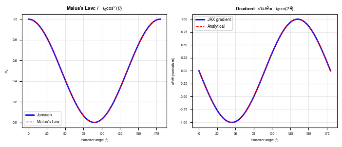
../_images/tutorials_Polarization_29_1.png

Max error in intensity: 2.22e-16
Max error in gradient: 4.44e-16

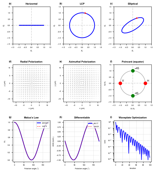
Publication Figure¶

Combined figure showing:

(a-c) Jones vector polarization ellipses
(d-e) Cylindrical vector beams
1. Poincaré sphere
(g-h) Malus’s law and gradient
1. Waveplate optimization

In [19]:

import string

fig = plt.figure(figsize=(7, 8))
gs = mpgs.GridSpec(3, 3, figure=fig, hspace=0.4, wspace=0.35)

subfig_idx = 0
def get_label():
    global subfig_idx
    label = f'({string.ascii_lowercase[subfig_idx]})'
    subfig_idx += 1
    return label

# Row 1: Polarization states (ellipses)
ellipse_states = [
    (1+0j, 0+0j, 'Horizontal'),
    (1+0j, 1j, 'LCP'),
    (1+0j, 0.5+0.5j, 'Elliptical')
]

for idx, (Ex, Ey, title) in enumerate(ellipse_states):
    ax = fig.add_subplot(gs[0, idx])
    norm = np.sqrt(abs(Ex)**2 + abs(Ey)**2)
    plot_polarization_state(ax, Ex/norm, Ey/norm, title)
    ax.text(-0.1, 1.05, get_label(), transform=ax.transAxes, fontweight='bold', va='bottom')

# Row 2: CVB and Poincare
# Radial polarization quiver
ax = fig.add_subplot(gs[1, 0])
radial = radially_polarized_beam(wavelength, dx, grid_size, beam_radius=beam_radius)
ex, ey = radial.field[..., 0], radial.field[..., 1]
ny, nx = ex.shape
step = 12
y_idx, x_idx = jnp.mgrid[step//2:ny:step, step//2:nx:step]
x_coords = (x_idx - nx/2) * dx * 1e6
y_coords = (y_idx - ny/2) * dx * 1e6
u = jnp.real(ex[y_idx, x_idx])
v = jnp.real(ey[y_idx, x_idx])
ax.quiver(x_coords, y_coords, u, v, pivot='mid', scale=20)
ax.set_xlim(-12, 12)
ax.set_ylim(-12, 12)
ax.set_aspect('equal')
ax.set_xlabel('x (μm)')
ax.set_ylabel('y (μm)')
ax.set_title('Radial Polarization')
ax.text(-0.1, 1.05, get_label(), transform=ax.transAxes, fontweight='bold', va='bottom')

# Azimuthal polarization quiver
ax = fig.add_subplot(gs[1, 1])
azimuthal = azimuthally_polarized_beam(wavelength, dx, grid_size, beam_radius=beam_radius)
ex, ey = azimuthal.field[..., 0], azimuthal.field[..., 1]
u = jnp.real(ex[y_idx, x_idx])
v = jnp.real(ey[y_idx, x_idx])
ax.quiver(x_coords, y_coords, u, v, pivot='mid', scale=20)
ax.set_xlim(-12, 12)
ax.set_ylim(-12, 12)
ax.set_aspect('equal')
ax.set_xlabel('x (μm)')
ax.set_ylabel('y (μm)')
ax.set_title('Azimuthal Polarization')
ax.text(-0.1, 1.05, get_label(), transform=ax.transAxes, fontweight='bold', va='bottom')

# Poincare sphere (2D projection)
ax = fig.add_subplot(gs[1, 2])
theta_circle = np.linspace(0, 2*np.pi, 100)
ax.plot(np.cos(theta_circle), np.sin(theta_circle), 'k-', alpha=0.3)
ax.axhline(0, color='gray', linestyle='--', alpha=0.3)
ax.axvline(0, color='gray', linestyle='--', alpha=0.3)

# Plot states (S1 vs S2 projection - equator of Poincare sphere)
poincare_states = [
    (1, 0, 'H', 'red'),
    (-1, 0, 'V', 'red'),
    (0, 1, '+45', 'green'),
    (0, -1, '-45', 'green'),
]
for s1, s2, label, color in poincare_states:
    ax.scatter(s1, s2, s=80, c=color, marker='o', zorder=5)
    ax.annotate(label, (s1, s2), xytext=(5, 5), textcoords='offset points', fontsize=8)

ax.set_xlabel('$S_1/S_0$')
ax.set_ylabel('$S_2/S_0$')
ax.set_title('Poincaré (equator)')
ax.set_aspect('equal')
ax.set_xlim(-1.5, 1.5)
ax.set_ylim(-1.5, 1.5)
ax.text(-0.1, 1.05, get_label(), transform=ax.transAxes, fontweight='bold', va='bottom')

# Row 3: Malus's law and optimization
ax = fig.add_subplot(gs[2, 0])
ax.plot(jnp.degrees(angles), intensities/I0, 'b-', linewidth=2, label='Janssen')
ax.plot(jnp.degrees(angles), jnp.cos(angles)**2, 'r--', linewidth=1, label='$\cos^2\\theta$')
ax.set_xlabel('Polarizer angle (°)')
ax.set_ylabel('$I/I_0$')
ax.set_title("Malus's Law")
ax.legend(loc='upper right', fontsize=5)
ax.grid(True, alpha=0.3)
ax.text(-0.1, 1.05, get_label(), transform=ax.transAxes, fontweight='bold', va='bottom')

ax = fig.add_subplot(gs[2, 1])
ax.plot(jnp.degrees(angles), gradients/I0, 'b-', linewidth=2, label='JAX $\\nabla$')
ax.plot(jnp.degrees(angles), -jnp.sin(2*angles), 'r--', linewidth=1, label='$-\sin 2\\theta$')
ax.set_xlabel('Polarizer angle (°)')
ax.set_ylabel('$\partial I/\partial\\theta$ (norm.)')
ax.set_title('Differentiable')
ax.legend(loc='upper right', fontsize=5)
ax.grid(True, alpha=0.3)
ax.text(-0.1, 1.05, get_label(), transform=ax.transAxes, fontweight='bold', va='bottom')

ax = fig.add_subplot(gs[2, 2])
ax.semilogy(loss_history, 'b-', linewidth=1.5)
ax.set_xlabel('Iteration')
ax.set_ylabel('Loss')
ax.set_title('Waveplate Optimization')
ax.grid(True, alpha=0.3)
ax.text(-0.1, 1.05, get_label(), transform=ax.transAxes, fontweight='bold', va='bottom')

plt.savefig('Figures/polarization_publication_figure.pdf', bbox_inches='tight',
            facecolor='white', edgecolor='none')
plt.savefig('Figures/polarization_publication_figure.png', dpi=300, bbox_inches='tight',
            facecolor='white', edgecolor='none')
plt.show()

<>:91: SyntaxWarning: invalid escape sequence '\c'
<>:101: SyntaxWarning: invalid escape sequence '\s'
<>:103: SyntaxWarning: invalid escape sequence '\p'
<>:91: SyntaxWarning: invalid escape sequence '\c'
<>:101: SyntaxWarning: invalid escape sequence '\s'
<>:103: SyntaxWarning: invalid escape sequence '\p'
/tmp/ipykernel_2057486/2956269917.py:91: SyntaxWarning: invalid escape sequence '\c'
  ax.plot(jnp.degrees(angles), jnp.cos(angles)**2, 'r--', linewidth=1, label='$\cos^2\\theta$')
/tmp/ipykernel_2057486/2956269917.py:101: SyntaxWarning: invalid escape sequence '\s'
  ax.plot(jnp.degrees(angles), -jnp.sin(2*angles), 'r--', linewidth=1, label='$-\sin 2\\theta$')
/tmp/ipykernel_2057486/2956269917.py:103: SyntaxWarning: invalid escape sequence '\p'
  ax.set_ylabel('$\partial I/\partial\\theta$ (norm.)')

../_images/tutorials_Polarization_31_1.png

Summary¶

This tutorial demonstrated:

Jones Calculus (coherent, fully polarized light)¶

Jones vectors: 2-component complex vectors representing polarization state
Jones matrices: 2×2 matrices for polarizers, waveplates
Cylindrical vector beams: Spatially varying polarization (radial, azimuthal)
Generalized CVB: Higher-order beams with multiple polarization singularities

Mueller-Stokes Calculus (partially polarized light)¶

Stokes vectors: 4-component real vectors with measurable intensities
Mueller matrices: 4×4 matrices including depolarizers
Poincaré sphere: Geometric visualization of polarization states

Differentiable Polarization Optics¶

Gradient computation: JAX enables \(\partial I / \partial \theta\) automatically
Parameter optimization: Recover waveplate angles from target polarization
Malus’s law verification: Exact match with analytical theory

Key Functions¶

Function	Description
`x_polarized_beam()`, `y_polarized_beam()`	Linear polarization
`circular_polarized_beam()`	RCP/LCP
`radially_polarized_beam()`	Radial CVB
`azimuthally_polarized_beam()`	Azimuthal CVB
`generalized_cylindrical_vector_beam()`	Higher-order CVB
`polarizer_jones()`	Linear polarizer (Jones)
`quarter_waveplate()`, `half_waveplate()`	Waveplates
`jones_to_stokes()`	Convert Jones → Stokes
`mueller_linear_polarizer()`	Mueller matrix for polarizer