Partial Coherence in Wave Optics¶

This tutorial covers partial coherence modeling in Janssen, demonstrating both spatial and temporal coherence effects and their differentiable implementation.

Overview¶

Real optical sources are never perfectly coherent:

LEDs have broad spectra and extended emitting areas
Synchrotron sources exhibit anisotropic spatial coherence
Lasers suffer from mode noise and finite linewidth

Modeling these effects requires moving beyond the single complex field \(E(x,y)\) to a statistical description of field correlations. This tutorial covers:

Spatial coherence: Extended sources and the van Cittert-Zernike theorem
Temporal coherence: Finite bandwidth and chromatic effects
Coherent mode decomposition: Efficient representation via Mercer’s theorem
Differentiability: Gradient-based recovery of coherence parameters

In [1]:

import jax
import jax.numpy as jnp
import matplotlib.pyplot as plt
import matplotlib.gridspec as gridspec
import numpy as np
import optax

import janssen as jns
from janssen.cohere import (
    gaussian_coherence_kernel,
    jinc_coherence_kernel,
    coherence_width_from_source,
    gaussian_spectrum,
    lorentzian_spectrum,
    coherence_length,
    gaussian_schell_model_modes,
    hermite_gaussian_modes,
    effective_mode_count,
    propagate_coherent_modes,
    propagate_and_focus_modes,
    intensity_from_modes,
    led_source,
)
from janssen.models import collimated_gaussian
from janssen.prop import angular_spectrum_prop

# Configure matplotlib for publication figures
plt.rcParams['font.family'] = 'sans-serif'
plt.rcParams['font.sans-serif'] = ['TeX Gyre Heros']
plt.rcParams['mathtext.fontset'] = 'custom'
plt.rcParams['mathtext.rm'] = 'TeX Gyre Heros'
plt.rcParams['mathtext.it'] = 'TeX Gyre Heros:italic'
plt.rcParams['mathtext.bf'] = 'TeX Gyre Heros:bold'

plt.rcParams['font.size'] = 6
plt.rcParams['axes.titlesize'] = 7
plt.rcParams['axes.titleweight'] = 'bold'
plt.rcParams['axes.labelsize'] = 5
plt.rcParams['xtick.labelsize'] = 5
plt.rcParams['ytick.labelsize'] = 5
plt.rcParams['legend.fontsize'] = 6
plt.rcParams['figure.titlesize'] = 7

Setup: Physical Parameters¶

In [2]:

# Physical parameters
wavelength = 633e-9  # HeNe laser, 633 nm
dx = 1e-6  # 1 um pixel size
grid_size = (256, 256)
beam_width = 100e-6  # 100 um beam width

# Derived quantities
physical_size = grid_size[0] * dx
extent_um = [-physical_size/2*1e6, physical_size/2*1e6,
             -physical_size/2*1e6, physical_size/2*1e6]

print(f"Wavelength: {wavelength*1e9:.0f} nm")
print(f"Grid: {grid_size[0]}x{grid_size[1]}, dx = {dx*1e6:.1f} um")
print(f"Physical extent: {physical_size*1e3:.2f} mm")

Wavelength: 633 nm
Grid: 256x256, dx = 1.0 um
Physical extent: 0.26 mm

Part I: Spatial Coherence¶

1.1 The Mutual Intensity¶

For quasi-monochromatic light, the mutual intensity describes correlations between field values at two points:

\[J(\mathbf{r}_1, \mathbf{r}_2) = \langle E^*(\mathbf{r}_1) E(\mathbf{r}_2) \rangle\]

The complex degree of coherence normalizes this:

\[\mu(\mathbf{r}_1, \mathbf{r}_2) = \frac{J(\mathbf{r}_1, \mathbf{r}_2)}{\sqrt{I(\mathbf{r}_1) I(\mathbf{r}_2)}}\]

where:

\(|\mu| = 1\): Fully coherent
\(|\mu| = 0\): Completely incoherent
\(0 < |\mu| < 1\): Partially coherent

1.2 Van Cittert-Zernike Theorem¶

For an extended incoherent source, the mutual intensity in the far field is the Fourier transform of the source intensity:

\[J(\mathbf{r}_1, \mathbf{r}_2) \propto \mathcal{F}\{I_{\text{source}}\}(\mathbf{r}_1 - \mathbf{r}_2)\]

A circular source of diameter \(D\) at distance \(z\) produces a jinc-shaped coherence function:

\[\mu(\Delta r) = 2\frac{J_1(\pi D \Delta r / \lambda z)}{\pi D \Delta r / \lambda z}\]

with coherence width \(\sigma_c \approx 0.44 \lambda z / D\).

In [3]:

# Compare coherence kernels
coherence_widths = [10e-6, 30e-6, 100e-6]  # 10, 30, 100 um

fig, axes = plt.subplots(2, 3, figsize=(7, 4.5))

for idx, sigma_c in enumerate(coherence_widths):
    # Gaussian kernel
    kernel_gauss = gaussian_coherence_kernel(
        grid_size=grid_size, dx=dx, coherence_width=sigma_c
    )

    # Jinc kernel (van Cittert-Zernike)
    # Calculate source diameter that gives this coherence width
    prop_distance = 0.1  # 10 cm
    source_diameter = 0.44 * wavelength * prop_distance / sigma_c
    kernel_jinc = jinc_coherence_kernel(
        grid_size=grid_size, dx=dx,
        source_diameter=source_diameter,
        wavelength=wavelength,
        propagation_distance=prop_distance
    )

    # Plot 2D kernel
    ax = axes[0, idx]
    im = ax.imshow(kernel_gauss, cmap='viridis', extent=extent_um, vmin=0, vmax=1)
    ax.set_title(f'$\\sigma_c$ = {sigma_c*1e6:.0f} \u03bcm')
    ax.set_xlabel('$\\Delta x$ (\u03bcm)')
    if idx == 0:
        ax.set_ylabel('$\\Delta y$ (\u03bcm)')
    ax.set_xlim(-100, 100)
    ax.set_ylim(-100, 100)

    # Plot 1D slice comparison
    ax = axes[1, idx]
    center = grid_size[0] // 2
    x_um = (jnp.arange(grid_size[1]) - center) * dx * 1e6

    ax.plot(x_um, kernel_gauss[center, :], 'b-', linewidth=1.5, label='Gaussian')
    ax.plot(x_um, kernel_jinc[center, :], 'r--', linewidth=1.5, label='Jinc (vCZ)')
    ax.set_xlabel('$\\Delta x$ (\u03bcm)')
    ax.set_ylabel('$|\\mu(\\Delta r)|$')
    ax.set_xlim(-100, 100)
    ax.set_ylim(-0.3, 1.1)
    ax.axhline(0, color='gray', linestyle=':', linewidth=0.5)
    ax.legend(loc='upper right', fontsize=5)
    ax.grid(True, alpha=0.3)

axes[0, 0].text(-0.15, 1.05, '(a)', transform=axes[0, 0].transAxes, fontweight='bold')
axes[0, 1].text(-0.15, 1.05, '(b)', transform=axes[0, 1].transAxes, fontweight='bold')
axes[0, 2].text(-0.15, 1.05, '(c)', transform=axes[0, 2].transAxes, fontweight='bold')
axes[1, 0].text(-0.15, 1.05, '(d)', transform=axes[1, 0].transAxes, fontweight='bold')
axes[1, 1].text(-0.15, 1.05, '(e)', transform=axes[1, 1].transAxes, fontweight='bold')
axes[1, 2].text(-0.15, 1.05, '(f)', transform=axes[1, 2].transAxes, fontweight='bold')

plt.tight_layout()
plt.savefig('Figures/coherence_spatial_kernels.pdf', bbox_inches='tight')
plt.savefig('Figures/coherence_spatial_kernels.png', dpi=300, bbox_inches='tight')
plt.show()

print(f"\nVan Cittert-Zernike relationship:")
print(f"  sigma_c = 0.44 * lambda * z / D")
for sigma_c in coherence_widths:
    D = 0.44 * wavelength * prop_distance / sigma_c
    print(f"  sigma_c = {sigma_c*1e6:.0f} um -> D = {D*1e3:.2f} mm (at z = {prop_distance*100:.0f} cm)")

WARNING:2026-01-05 00:54:25,198:jax._src.xla_bridge:864: An NVIDIA GPU may be present on this machine, but a CUDA-enabled jaxlib is not installed. Falling back to cpu.


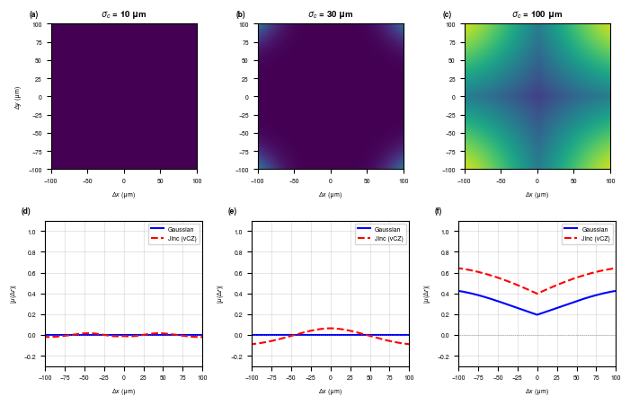
Van Cittert-Zernike relationship:
  sigma_c = 0.44 * lambda * z / D
  sigma_c = 10 um -> D = 2.79 mm (at z = 10 cm)
  sigma_c = 30 um -> D = 0.93 mm (at z = 10 cm)
  sigma_c = 100 um -> D = 0.28 mm (at z = 10 cm)

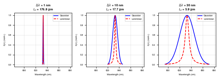
Part II: Temporal Coherence¶

2.1 Spectral Width and Coherence Length¶

Temporal coherence arises from finite spectral bandwidth. The coherence length is:

\[L_c = \frac{\lambda^2}{\Delta\lambda}\]

This determines the path-length difference over which interference is observable.

Source Type	Bandwidth	Coherence Length
HeNe laser	~1 pm	~400 m
LED	~30 nm	~13 \u03bcm
White light	~300 nm	~1 \u03bcm

In [4]:

# Compare spectral distributions
center_wavelength = 633e-9
bandwidths_nm = [1, 10, 30]  # nm
num_wavelengths = 101

fig, axes = plt.subplots(1, 3, figsize=(7, 2.5))

for idx, bw_nm in enumerate(bandwidths_nm):
    bw = bw_nm * 1e-9

    # Gaussian spectrum
    wls_g, weights_g = gaussian_spectrum(
        center_wavelength=center_wavelength,
        bandwidth_fwhm=bw,
        num_wavelengths=num_wavelengths
    )

    # Lorentzian spectrum
    wls_l, weights_l = lorentzian_spectrum(
        center_wavelength=center_wavelength,
        bandwidth_fwhm=bw,
        num_wavelengths=num_wavelengths
    )

    # Coherence length
    L_c = coherence_length(center_wavelength, bw)

    ax = axes[idx]
    wls_nm = wls_g * 1e9
    ax.plot(wls_nm, weights_g / jnp.max(weights_g), 'b-', linewidth=1.5, label='Gaussian')
    ax.plot(wls_nm, weights_l / jnp.max(weights_l), 'r--', linewidth=1.5, label='Lorentzian')
    ax.set_xlabel('Wavelength (nm)')
    ax.set_ylabel('S($\\lambda$) (norm.)')
    ax.set_title(f'$\\Delta\\lambda$ = {bw_nm} nm\n$L_c$ = {L_c*1e6:.1f} \u03bcm')
    ax.legend(loc='upper right', fontsize=5)
    ax.grid(True, alpha=0.3)
    ax.set_xlim(center_wavelength*1e9 - 50, center_wavelength*1e9 + 50)

plt.tight_layout()
plt.savefig('Figures/coherence_temporal_spectra.pdf', bbox_inches='tight')
plt.savefig('Figures/coherence_temporal_spectra.png', dpi=300, bbox_inches='tight')
plt.show()

Part III: Coherent Mode Decomposition¶

3.1 Mercer’s Theorem¶

Any partially coherent field can be decomposed into orthogonal coherent modes:

\[J(\mathbf{r}_1, \mathbf{r}_2) = \sum_n \lambda_n \phi_n^*(\mathbf{r}_1) \phi_n(\mathbf{r}_2)\]

where:

\(\phi_n\) are orthonormal modes
\(\lambda_n\) are modal weights (eigenvalues)

The total intensity is an incoherent sum:

\[I(\mathbf{r}) = \sum_n \lambda_n |\phi_n(\mathbf{r})|^2\]

3.2 Gaussian Schell-Model Source¶

For a Gaussian Schell-model (GSM) source with beam width \(\sigma_I\) and coherence width \(\sigma_c\):

The modes are Hermite-Gaussian functions
The eigenvalues are analytically known:

\[\lambda_n = \left(\frac{1-a}{1+a}\right) \left(\frac{a}{1+a}\right)^n, \quad a = \frac{\sigma_c}{\sigma_I}\]

The effective number of modes (participation ratio) is:

\[M_{\text{eff}} = \frac{(\sum_n \lambda_n)^2}{\sum_n \lambda_n^2}\]

In [5]:

# Generate Gaussian Schell-model modes for different coherence levels
coherence_ratios = [0.9, 0.5, 0.2]  # sigma_c / sigma_I
num_modes = 15

fig, axes = plt.subplots(3, 4, figsize=(9, 7))

for row, ratio in enumerate(coherence_ratios):
    sigma_c = ratio * beam_width

    # Generate GSM modes
    mode_set = gaussian_schell_model_modes(
        wavelength=wavelength,
        dx=dx,
        grid_size=grid_size,
        beam_width=beam_width,
        coherence_width=sigma_c,
        num_modes=num_modes
    )

    M_eff = effective_mode_count(mode_set)

    # Plot first 3 modes
    for col in range(3):
        ax = axes[row, col]
        mode_intensity = jnp.abs(mode_set.modes[col])**2
        im = ax.imshow(mode_intensity, cmap='inferno', extent=extent_um)
        ax.set_xlim(-150, 150)
        ax.set_ylim(-150, 150)
        if row == 0:
            ax.set_title(f'Mode {col}')
        if col == 0:
            ax.set_ylabel(f'$\\sigma_c/\\sigma_I$ = {ratio}\n$M_{{eff}}$ = {M_eff:.1f}')
        ax.set_xticks([])
        ax.set_yticks([])

    # Plot eigenvalue spectrum
    ax = axes[row, 3]
    ax.bar(range(num_modes), mode_set.weights, color='steelblue', edgecolor='navy')
    ax.set_xlabel('Mode index')
    ax.set_ylabel('Weight $\\lambda_n$')
    ax.set_ylim(0, 1)
    ax.grid(True, alpha=0.3)
    if row == 0:
        ax.set_title('Eigenvalue Spectrum')

plt.tight_layout()
plt.savefig('Figures/coherence_gsm_modes.pdf', bbox_inches='tight')
plt.savefig('Figures/coherence_gsm_modes.png', dpi=300, bbox_inches='tight')
plt.show()

print("\nEffective mode count vs. coherence ratio:")
for ratio in coherence_ratios:
    sigma_c = ratio * beam_width
    mode_set = gaussian_schell_model_modes(
        wavelength=wavelength, dx=dx, grid_size=grid_size,
        beam_width=beam_width, coherence_width=sigma_c, num_modes=num_modes
    )
    M_eff = effective_mode_count(mode_set)
    print(f"  sigma_c/sigma_I = {ratio:.1f} -> M_eff = {M_eff:.2f}")


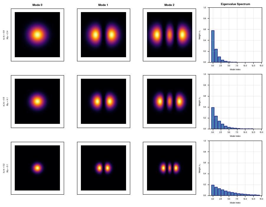
Effective mode count vs. coherence ratio:
  sigma_c/sigma_I = 0.9 -> M_eff = 2.44
  sigma_c/sigma_I = 0.5 -> M_eff = 4.12
  sigma_c/sigma_I = 0.2 -> M_eff = 9.09

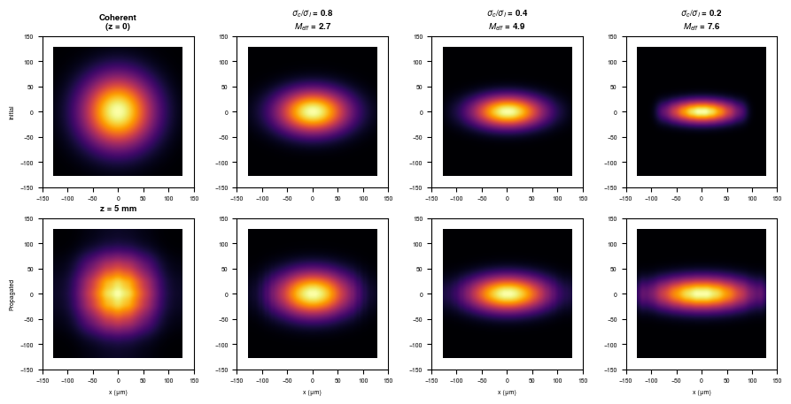
3.3 Propagation of Partially Coherent Fields¶

Each coherent mode propagates independently. The final intensity is the incoherent sum of propagated mode intensities.

This is implemented efficiently using jax.vmap for parallel propagation of all modes.

In [6]:

# Compare fully coherent vs partially coherent propagation
prop_distance = 5e-3  # 5 mm

# Fully coherent Gaussian beam
coherent_beam = collimated_gaussian(
    wavelength=wavelength, dx=dx, grid_size=grid_size,
    waist=beam_width, z_position=0.0
)
coherent_propagated = angular_spectrum_prop(coherent_beam, prop_distance)
I_coherent = jnp.abs(coherent_propagated.field)**2

# Partially coherent (GSM) beam with different coherence levels
coherence_levels = [0.8, 0.4, 0.2]

fig, axes = plt.subplots(2, 4, figsize=(9, 4.5))

# Top row: Initial intensity
ax = axes[0, 0]
I_initial = jnp.abs(coherent_beam.field)**2
ax.imshow(I_initial, cmap='inferno', extent=extent_um)
ax.set_title('Coherent\n(z = 0)')
ax.set_xlim(-150, 150)
ax.set_ylim(-150, 150)
ax.set_ylabel('Initial')

for idx, ratio in enumerate(coherence_levels):
    sigma_c = ratio * beam_width
    mode_set = gaussian_schell_model_modes(
        wavelength=wavelength, dx=dx, grid_size=grid_size,
        beam_width=beam_width, coherence_width=sigma_c, num_modes=10
    )
    I_initial_pc = intensity_from_modes(mode_set)

    ax = axes[0, idx+1]
    ax.imshow(I_initial_pc, cmap='inferno', extent=extent_um)
    M_eff = effective_mode_count(mode_set)
    ax.set_title(f'$\\sigma_c/\\sigma_I$ = {ratio}\n$M_{{eff}}$ = {M_eff:.1f}')
    ax.set_xlim(-150, 150)
    ax.set_ylim(-150, 150)

# Bottom row: After propagation
ax = axes[1, 0]
ax.imshow(I_coherent, cmap='inferno', extent=extent_um)
ax.set_title(f'z = {prop_distance*1e3:.0f} mm')
ax.set_xlim(-150, 150)
ax.set_ylim(-150, 150)
ax.set_ylabel('Propagated')
ax.set_xlabel('x (μm)')

for idx, ratio in enumerate(coherence_levels):
    sigma_c = ratio * beam_width
    mode_set = gaussian_schell_model_modes(
        wavelength=wavelength, dx=dx, grid_size=grid_size,
        beam_width=beam_width, coherence_width=sigma_c, num_modes=10
    )

    # Propagate modes
    mode_set_prop = propagate_coherent_modes(mode_set, prop_distance)
    I_prop = intensity_from_modes(mode_set_prop)

    ax = axes[1, idx+1]
    ax.imshow(I_prop, cmap='inferno', extent=extent_um)
    ax.set_xlim(-150, 150)
    ax.set_ylim(-150, 150)
    ax.set_xlabel('x (μm)')

plt.tight_layout()
plt.savefig('Figures/coherence_propagation_comparison.pdf', bbox_inches='tight')
plt.savefig('Figures/coherence_propagation_comparison.png', dpi=300, bbox_inches='tight')
plt.show()

Part IV: Differentiable Partial Coherence¶

4.1 Why Differentiability Matters¶

Because Janssen implements coherent mode propagation using JAX, we can compute gradients with respect to coherence parameters. This enables:

Coherence recovery: Estimate source coherence from measured intensity patterns
Joint optimization: Recover both object and coherence in ptychography
Sensitivity analysis: How do results depend on coherence assumptions?

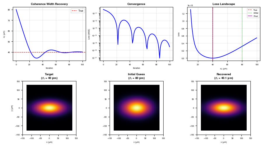
4.2 Example: Recovering Coherence Width from Propagated Intensity¶

Given a measured intensity pattern after propagation, can we recover the source coherence width?

In [7]:

# Define forward model: coherence width -> propagated intensity
prop_distance_opt = 5e-3  # 5 mm
num_modes_opt = 10

def forward_model(coherence_width):
    """Compute propagated intensity for given coherence width."""
    mode_set = gaussian_schell_model_modes(
        wavelength=wavelength,
        dx=dx,
        grid_size=grid_size,
        beam_width=beam_width,
        coherence_width=coherence_width,
        num_modes=num_modes_opt
    )
    mode_set_prop = propagate_coherent_modes(mode_set, prop_distance_opt)
    intensity = intensity_from_modes(mode_set_prop)
    return intensity

# Generate "ground truth" target with known coherence
true_coherence_width = 40e-6  # 40 um
I_target = forward_model(true_coherence_width)

print(f"True coherence width: {true_coherence_width*1e6:.0f} um")
print(f"Propagation distance: {prop_distance_opt*1e3:.0f} mm")

True coherence width: 40 um
Propagation distance: 5 mm

In [8]:

# Define loss function and compute gradient
def loss_fn(coherence_width):
    """MSE between predicted and target intensity."""
    I_pred = forward_model(coherence_width)
    return jnp.mean((I_pred - I_target)**2)

# Compute gradient with JAX
grad_loss = jax.grad(loss_fn)

# Test at a few points
test_widths = [20e-6, 40e-6, 60e-6, 80e-6]
print("\nLoss and gradient at different coherence widths:")
print(f"{'sigma_c (um)':<15} {'Loss':<15} {'dL/d(sigma_c)':<15}")
print("-" * 45)
for w in test_widths:
    loss = float(loss_fn(w))
    grad = float(grad_loss(w))
    print(f"{w*1e6:<15.0f} {loss:<15.6f} {grad:<15.6f}")


Loss and gradient at different coherence widths:
sigma_c (um)    Loss            dL/d(sigma_c)
---------------------------------------------
20              0.000000        -0.000003
40              0.000000        -0.000000
60              0.000000        0.000001
80              0.000000        0.000001

In [9]:

# Gradient-based optimization to recover coherence width
initial_guess = 80e-6  # Start with wrong value (80 um instead of 40 um)

optimizer = optax.adam(learning_rate=2e-6)
params = jnp.array(initial_guess)
opt_state = optimizer.init(params)

n_iterations = 100
coherence_history = [float(params)]
loss_history = [float(loss_fn(params))]

print(f"Recovering coherence width from propagated intensity...")
print(f"True value: {true_coherence_width*1e6:.0f} um")
print(f"Initial guess: {initial_guess*1e6:.0f} um")
print(f"\nOptimization progress:")

for i in range(n_iterations):
    grad = grad_loss(params)
    updates, opt_state = optimizer.update(grad, opt_state)
    params = optax.apply_updates(params, updates)

    # Ensure params stay positive
    params = jnp.maximum(params, 1e-6)

    coherence_history.append(float(params))
    loss_history.append(float(loss_fn(params)))

    if (i + 1) % 20 == 0:
        print(f"  Iter {i+1:3d}: sigma_c = {params*1e6:.2f} um, loss = {loss_history[-1]:.2e}")

print(f"\nFinal estimate: {params*1e6:.2f} um")
print(f"True value: {true_coherence_width*1e6:.0f} um")
print(f"Error: {abs(params - true_coherence_width)*1e6:.2f} um ({abs(params - true_coherence_width)/true_coherence_width*100:.1f}%)")

Recovering coherence width from propagated intensity...
True value: 40 um
Initial guess: 80 um

Optimization progress:
  Iter  20: sigma_c = 42.60 um, loss = 2.20e-13
  Iter  40: sigma_c = 37.73 um, loss = 1.76e-13
  Iter  60: sigma_c = 41.10 um, loss = 4.04e-14
  Iter  80: sigma_c = 39.63 um, loss = 4.64e-15
  Iter 100: sigma_c = 40.09 um, loss = 2.86e-16

Final estimate: 40.09 um
True value: 40 um
Error: 0.09 um (0.2%)

In [10]:

# Plot optimization results
fig, axes = plt.subplots(2, 3, figsize=(9, 5))

# Top row: Convergence
ax = axes[0, 0]
ax.plot([w*1e6 for w in coherence_history], 'b-', linewidth=1.5)
ax.axhline(true_coherence_width*1e6, color='r', linestyle='--', linewidth=1, label='True')
ax.set_xlabel('Iteration')
ax.set_ylabel('$\\sigma_c$ (\u03bcm)')
ax.set_title('Coherence Width Recovery')
ax.legend(loc='upper right')
ax.grid(True, alpha=0.3)

ax = axes[0, 1]
ax.semilogy(loss_history, 'b-', linewidth=1.5)
ax.set_xlabel('Iteration')
ax.set_ylabel('Loss (MSE)')
ax.set_title('Convergence')
ax.grid(True, alpha=0.3)

# Loss landscape
ax = axes[0, 2]
sigma_range = jnp.linspace(10e-6, 100e-6, 50)
losses = [float(loss_fn(s)) for s in sigma_range]
ax.plot(sigma_range*1e6, losses, 'b-', linewidth=1.5)
ax.axvline(true_coherence_width*1e6, color='r', linestyle='--', linewidth=1, label='True')
ax.axvline(initial_guess*1e6, color='g', linestyle=':', linewidth=1, label='Initial')
ax.axvline(params*1e6, color='purple', linestyle='-', linewidth=1, label='Final')
ax.set_xlabel('$\\sigma_c$ (\u03bcm)')
ax.set_ylabel('Loss')
ax.set_title('Loss Landscape')
ax.legend(loc='upper right', fontsize=5)
ax.grid(True, alpha=0.3)

# Bottom row: Intensity comparisons
I_initial = forward_model(initial_guess)
I_final = forward_model(params)

ax = axes[1, 0]
ax.imshow(I_target, cmap='inferno', extent=extent_um)
ax.set_title(f'Target\n($\\sigma_c$ = {true_coherence_width*1e6:.0f} \u03bcm)')
ax.set_xlim(-150, 150)
ax.set_ylim(-150, 150)
ax.set_xlabel('x (\u03bcm)')
ax.set_ylabel('y (\u03bcm)')

ax = axes[1, 1]
ax.imshow(I_initial, cmap='inferno', extent=extent_um)
ax.set_title(f'Initial Guess\n($\\sigma_c$ = {initial_guess*1e6:.0f} \u03bcm)')
ax.set_xlim(-150, 150)
ax.set_ylim(-150, 150)
ax.set_xlabel('x (\u03bcm)')

ax = axes[1, 2]
ax.imshow(I_final, cmap='inferno', extent=extent_um)
ax.set_title(f'Recovered\n($\\sigma_c$ = {params*1e6:.1f} \u03bcm)')
ax.set_xlim(-150, 150)
ax.set_ylim(-150, 150)
ax.set_xlabel('x (\u03bcm)')

plt.tight_layout()
plt.savefig('Figures/coherence_optimization.pdf', bbox_inches='tight')
plt.savefig('Figures/coherence_optimization.png', dpi=300, bbox_inches='tight')
plt.show()

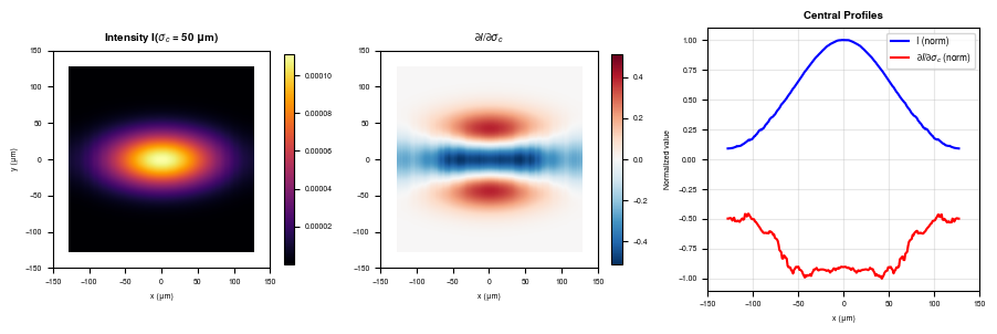
4.3 Gradient Visualization¶

We can visualize how the propagated intensity depends on coherence width by computing the spatial gradient map \(\partial I(\mathbf{r}) / \partial \sigma_c\).

In [11]:

# Compute gradient of intensity with respect to coherence width
def intensity_at_coherence(coherence_width):
    return forward_model(coherence_width)

# Use finite difference for spatial gradient map
eps = 1e-7
sigma_test = 50e-6
I_plus = intensity_at_coherence(sigma_test + eps)
I_minus = intensity_at_coherence(sigma_test - eps)
dI_dsigma = (I_plus - I_minus) / (2 * eps)

fig, axes = plt.subplots(1, 3, figsize=(9, 3))

# Intensity
ax = axes[0]
I_test = intensity_at_coherence(sigma_test)
im = ax.imshow(I_test, cmap='inferno', extent=extent_um)
ax.set_title(f'Intensity I($\\sigma_c$ = {sigma_test*1e6:.0f} \u03bcm)')
ax.set_xlabel('x (\u03bcm)')
ax.set_ylabel('y (\u03bcm)')
ax.set_xlim(-150, 150)
ax.set_ylim(-150, 150)
plt.colorbar(im, ax=ax, shrink=0.8)

# Gradient map
ax = axes[1]
vmax = jnp.max(jnp.abs(dI_dsigma))
im = ax.imshow(dI_dsigma, cmap='RdBu_r', extent=extent_um, vmin=-vmax, vmax=vmax)
ax.set_title('$\\partial I / \\partial \\sigma_c$')
ax.set_xlabel('x (\u03bcm)')
ax.set_xlim(-150, 150)
ax.set_ylim(-150, 150)
plt.colorbar(im, ax=ax, shrink=0.8)

# 1D profiles
ax = axes[2]
center = grid_size[0] // 2
x_um = (jnp.arange(grid_size[1]) - center) * dx * 1e6

ax.plot(x_um, I_test[center, :] / jnp.max(I_test), 'b-', linewidth=1.5, label='I (norm)')
ax.plot(x_um, dI_dsigma[center, :] / vmax, 'r-', linewidth=1.5, label='$\\partial I/\\partial\\sigma_c$ (norm)')
ax.set_xlabel('x (\u03bcm)')
ax.set_ylabel('Normalized value')
ax.set_title('Central Profiles')
ax.set_xlim(-150, 150)
ax.legend(loc='upper right', fontsize=6)
ax.grid(True, alpha=0.3)

plt.tight_layout()
plt.savefig('Figures/coherence_gradient_map.pdf', bbox_inches='tight')
plt.savefig('Figures/coherence_gradient_map.png', dpi=300, bbox_inches='tight')
plt.show()

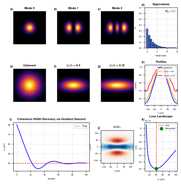
Publication Figure¶

Combined figure for the Janssen manuscript demonstrating partial coherence:

Row (a-c): Gaussian Schell-model modes 0, 1, 2 with eigenvalues — showing Hermite-Gaussian structure
Row (d-f): Focal intensity vs coherence width: σ_c = ∞ (coherent), σ_c = 2w₀, σ_c = w₀ — demonstrates speckle washing
Row (g-i): Differentiable demo: recover σ_c from blurred focal spot via gradient descent

In [12]:

import string

fig = plt.figure(figsize=(7, 7))
gs = gridspec.GridSpec(3, 4, figure=fig, hspace=0.4, wspace=0.35,
                       height_ratios=[1, 1, 1.2])

subfig_idx = 0
def get_label():
    global subfig_idx
    label = f'({string.ascii_lowercase[subfig_idx]})'
    subfig_idx += 1
    return label

# Row 1: GSM modes (high coherence case)
ratio_demo = 0.4
sigma_c_demo = ratio_demo * beam_width
mode_set_demo = gaussian_schell_model_modes(
    wavelength=wavelength, dx=dx, grid_size=grid_size,
    beam_width=beam_width, coherence_width=sigma_c_demo, num_modes=num_modes
)

for col in range(3):
    ax = fig.add_subplot(gs[0, col])
    mode_intensity = jnp.abs(mode_set_demo.modes[col])**2
    ax.imshow(mode_intensity, cmap='inferno', extent=extent_um)
    ax.set_xlim(-120, 120)
    ax.set_ylim(-120, 120)
    ax.set_title(f'Mode {col}')
    ax.set_xticks([])
    ax.set_yticks([])
    ax.text(-0.1, 1.05, get_label(), transform=ax.transAxes, fontweight='bold')

# Eigenvalue spectrum
ax = fig.add_subplot(gs[0, 3])
ax.bar(range(num_modes), mode_set_demo.weights, color='steelblue', edgecolor='navy')
ax.set_xlabel('Mode index')
ax.set_ylabel('$\\lambda_n$')
ax.set_title('Eigenvalues')
ax.set_ylim(0, 0.7)
ax.grid(True, alpha=0.3)
M_eff_demo = effective_mode_count(mode_set_demo)
ax.text(0.95, 0.95, f'$M_{{eff}}$ = {M_eff_demo:.1f}', transform=ax.transAxes,
        ha='right', va='top', fontsize=6)
ax.text(-0.1, 1.05, get_label(), transform=ax.transAxes, fontweight='bold')

# Row 2: Propagation comparison
prop_levels = [1.0, 0.4, 0.15]  # Fully coherent, partially, more partial

# Fully coherent
ax = fig.add_subplot(gs[1, 0])
I_coh_prop = jnp.abs(coherent_propagated.field)**2
ax.imshow(I_coh_prop, cmap='inferno', extent=extent_um)
ax.set_xlim(-120, 120)
ax.set_ylim(-120, 120)
ax.set_title('Coherent')
ax.set_xticks([])
ax.set_yticks([])
ax.text(-0.1, 1.05, get_label(), transform=ax.transAxes, fontweight='bold')

# Partially coherent cases
for idx, ratio in enumerate([0.4, 0.15]):
    ax = fig.add_subplot(gs[1, idx+1])
    sigma_c_prop = ratio * beam_width
    mode_set_prop = gaussian_schell_model_modes(
        wavelength=wavelength, dx=dx, grid_size=grid_size,
        beam_width=beam_width, coherence_width=sigma_c_prop, num_modes=10
    )
    mode_set_propagated = propagate_coherent_modes(mode_set_prop, prop_distance)
    I_prop = intensity_from_modes(mode_set_propagated)
    ax.imshow(I_prop, cmap='inferno', extent=extent_um)
    ax.set_xlim(-120, 120)
    ax.set_ylim(-120, 120)
    M_eff_prop = effective_mode_count(mode_set_prop)
    ax.set_title(f'$\\sigma_c/\\sigma_I$ = {ratio}')
    ax.set_xticks([])
    ax.set_yticks([])
    ax.text(-0.1, 1.05, get_label(), transform=ax.transAxes, fontweight='bold')

# Profile comparison
ax = fig.add_subplot(gs[1, 3])
center = grid_size[0] // 2
x_um = (jnp.arange(grid_size[1]) - center) * dx * 1e6

ax.plot(x_um, I_coh_prop[center, :] / jnp.max(I_coh_prop), 'b-',
        linewidth=1.5, label='Coherent')

for ratio, color in [(0.4, 'orange'), (0.15, 'red')]:
    sigma_c_prop = ratio * beam_width
    mode_set_prop = gaussian_schell_model_modes(
        wavelength=wavelength, dx=dx, grid_size=grid_size,
        beam_width=beam_width, coherence_width=sigma_c_prop, num_modes=10
    )
    mode_set_propagated = propagate_coherent_modes(mode_set_prop, prop_distance)
    I_prop = intensity_from_modes(mode_set_propagated)
    ax.plot(x_um, I_prop[center, :] / jnp.max(I_prop), color=color,
            linewidth=1.5, label=f'$\\sigma_c/\\sigma_I$ = {ratio}')

ax.set_xlabel('x (\u03bcm)')
ax.set_ylabel('I (norm.)')
ax.set_title('Profiles')
ax.set_xlim(-120, 120)
ax.legend(loc='upper right', fontsize=5)
ax.grid(True, alpha=0.3)
ax.text(-0.1, 1.05, get_label(), transform=ax.transAxes, fontweight='bold')

# Row 3: Optimization demo
# Coherence recovery
ax = fig.add_subplot(gs[2, 0:2])
ax.plot([w*1e6 for w in coherence_history], 'b-', linewidth=1.5)
ax.axhline(true_coherence_width*1e6, color='r', linestyle='--', linewidth=1, label='True')
ax.set_xlabel('Iteration')
ax.set_ylabel('$\\sigma_c$ (\u03bcm)')
ax.set_title('Coherence Width Recovery via Gradient Descent')
ax.legend(loc='upper right')
ax.grid(True, alpha=0.3)
ax.text(-0.05, 1.05, get_label(), transform=ax.transAxes, fontweight='bold')

# Gradient map
ax = fig.add_subplot(gs[2, 2])
vmax_pub = jnp.max(jnp.abs(dI_dsigma))
ax.imshow(dI_dsigma, cmap='RdBu_r', extent=extent_um, vmin=-vmax_pub, vmax=vmax_pub)
ax.set_xlim(-120, 120)
ax.set_ylim(-120, 120)
ax.set_title('$\\partial I / \\partial \\sigma_c$')
ax.set_xlabel('x (\u03bcm)')
ax.set_ylabel('y (\u03bcm)')
ax.text(-0.1, 1.05, get_label(), transform=ax.transAxes, fontweight='bold')

# Loss landscape
ax = fig.add_subplot(gs[2, 3])
ax.plot(sigma_range*1e6, losses, 'b-', linewidth=1.5)
ax.axvline(true_coherence_width*1e6, color='r', linestyle='--', linewidth=1, label='True')
ax.scatter([params*1e6], [loss_fn(params)], c='green', s=50, zorder=5, label='Recovered')
ax.set_xlabel('$\\sigma_c$ (\u03bcm)')
ax.set_ylabel('Loss')
ax.set_title('Loss Landscape')
ax.legend(loc='upper right', fontsize=5)
ax.grid(True, alpha=0.3)
ax.text(-0.1, 1.05, get_label(), transform=ax.transAxes, fontweight='bold')

plt.savefig('Figures/coherence_publication_figure.pdf', bbox_inches='tight',
            facecolor='white', edgecolor='none')
plt.savefig('Figures/coherence_publication_figure.png', dpi=300, bbox_inches='tight',
            facecolor='white', edgecolor='none')
plt.show()

Summary¶

This tutorial demonstrated:

Spatial Coherence¶

Mutual intensity \(J(\mathbf{r}_1, \mathbf{r}_2)\) describes field correlations
Van Cittert-Zernike theorem: Extended sources create spatial coherence patterns
Coherence kernels: Gaussian and jinc (for circular sources)

Temporal Coherence¶

Spectral bandwidth determines coherence length \(L_c = \lambda^2/\Delta\lambda\)
Spectral shapes: Gaussian, Lorentzian, blackbody distributions

Coherent Mode Decomposition¶

Mercer’s theorem: \(J = \sum_n \lambda_n \phi_n^* \phi_n\)
Gaussian Schell-model: Analytical Hermite-Gaussian modes
Effective mode count: Quantifies degree of partial coherence
Efficient propagation via vmap over modes

Differentiability¶

Gradient computation: JAX enables \(\partial I / \partial \sigma_c\) automatically
Coherence recovery: Gradient descent can recover source coherence from measurements
Joint optimization: Coherence parameters can be optimized alongside object/probe

Key Functions¶

Function	Description
`gaussian_coherence_kernel()`	Gaussian spatial coherence
`jinc_coherence_kernel()`	Van Cittert-Zernike for circular source
`gaussian_schell_model_modes()`	GSM source modes
`propagate_coherent_modes()`	Propagate mode set
`intensity_from_modes()`	Incoherent intensity sum
`effective_mode_count()`	Participation ratio